📐 Linear Regression

Linear regression is a supervised learning algorithm used to predict a continuous output variable based on one or more input features.

• It is widely used for prediction, forecasting, and as a baseline model.
• It assumes that the relationship between inputs and output is linear.

$$y = \theta_0 + \theta_1 x$$

When to Use Linear Regression

Linear regression is ideal for:

• Price prediction
• Trend analysis
• Baseline modeling
• Interpretable relationships
• Fast and simple forecasting

It is often used as a baseline before trying more complex models.

Key Assumptions

Linear regression works best when:

• The relationship is approximately linear
• Errors are independent
• Variance of errors is constant
• Residuals are normally distributed

Understanding these assumptions is important for reliable modeling.

---

🧮 Training Set $(x,y)$

Training Set is the Data that is fed to Leaning Algorithm.

The Learning function outputs a hypothesis function

$$X = \begin{bmatrix} 1 & x_1^{(1)} & \dots & x_n^{(1)} \\ 1 & x_1^{(2)} & \dots & x_n^{(2)} \\ \vdots & \vdots & & \vdots \\ 1 & x_1^{(m)} & \dots & x_n^{(m)} \end{bmatrix}$$

• $x$ = inputs
• $y$ = expected output
• $(x,y)$ = Row in Training Set: single training example
• $(Xi,Yi)$ = i-th training example
• $m$ = Number of training examples - rows in training set
• $n$ = Number of features - columns in training set

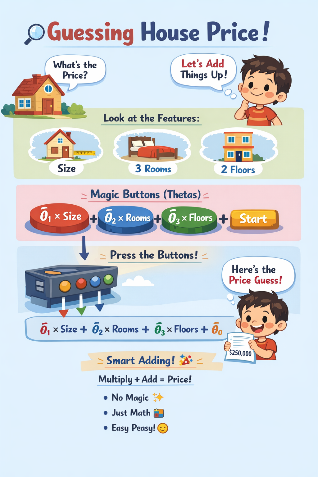
Example: 🏠 House price

Size (x₁)	Rooms (x₂)	Price (y)
50	1	150
80	2	230
120	3	310

• 📏 $x_1$ → size of house
• 🛏 $x_2$ → number of Rooms
• $m$ = 3 training examples
• $n$ = 2 features

In machine learning, it’s often not who has the best algorithm, but who has the most data.

Testing several learning algorithms while increasing the training set size.

The key findings:

1. Different algorithms often performed similarly.
2. Performance improved steadily as training set size increased.
3. An “inferior” algorithm with more data often outperformed a “superior” algorithm with less data.

More data helps when:

$$\text{Sufficient features} + \text{Low bias model} + \text{Large dataset} \Rightarrow \text{Low bias and low variance}$$

1. Use a rich model → low bias
2. Use a massive dataset → low variance

If both are true, then:

• Training error is small
• Test error is close to training error
• Test error is also small

1. Your input features $x$ must contain enough features to predict $y$ accurately.

Given only the features $x$, could a human expert confidently predict $y$?

• If yes, then the problem likely has enough signal.
• If not, no amount of data will fix it.

2. Use a High-Capacity (Low-Bias) Model

You need a powerful learning algorithm, such as:

• Logistic regression with many features
• Linear regression with many features
• Neural networks with many hidden units These models have many parameters and can represent complex functions.

This helps ensure low bias.

3. Use a Very Large Training Set

If:

• The model has many parameters
• The training set is much larger than the number of parameters

Then overfitting becomes less likely.

This helps reduce variance.

---

💡 Hypothesis $h_\theta(x)$

Function that maps input $x$ to output $y$ is called Hypothesis function.

Supervised learning works like this:

Training Set → Learning Algorithm → Hypothesis Function

The algorithm outputs a function called: h (hypothesis)

• $h$ = hypothesis, trained Algo that can map $Y$ to $Y$

$$h_\theta(x) = \theta^T x$$

Finding $\theta$

Our goal is to find the best values of $\theta$ that minimize prediction error.

1. Single Variable Linear Regression : $h_\theta(x)$

Linear regression is method of finding a Continues linear relationship between Y and X

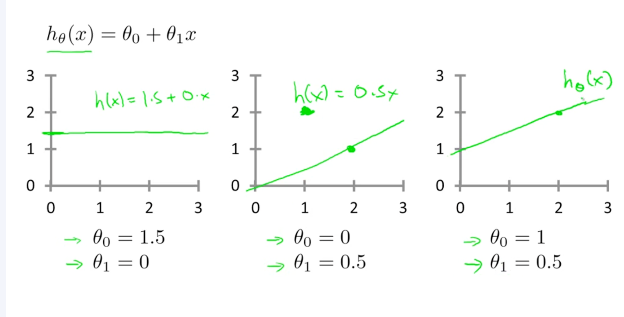
When there is only one feature, the model is:

$$y = \theta_0 + \theta_1 x$$ $$h_\theta(x) = \theta_0 + \theta_1 x$$

This represents a straight line, where:

• $y$ = is the predicted value
• $x$ = is the input feature
• $\theta_0$ = is the Y intercept
• $\theta_1$ = is the slope of line

Example:

• $\theta_0 = 0$ → line passes through origin

• $\theta_1 = 0$ → horizontal line

  

2. Multi Variate Linear Regression: $h_\theta(x)$

Linear regression with multiple variables

For multiple features:

$$h_\theta(x) = \theta_0 + \theta_1 x_1 + \dots + \theta_n x_n$$

Matrix form:

$$X = \begin{bmatrix} 1 & 50 & 1 \\ 1 & 80 & 2 \\ 1 & 120 & 3 \end{bmatrix}$$

Parameter Vector

$$\theta = \begin{bmatrix} \theta_0 \\ \theta_1 \\ \theta_2 \end{bmatrix}$$

Target Vector

$$y = \begin{bmatrix} 150 \\ 230 \\ 310 \end{bmatrix}$$

This form is computationally efficient.

Calculating Hypothesis Function

Using Closed-form solution:

$\theta = (X^T X)^{-1} X^T y$

• $\theta_0 \approx 20$ : Base price of house
• $\theta_1 \approx 2$ : Price increase per unit size
• $\theta_2 \approx 30$ : Price increase per additional room

Final Hypothesis Function:

$$House Price = 20 + (2) \cdot Size + (30) \cdot Rooms$$

Model Inference

Test For:

• Size = 100
• Rooms = 2

$$Price = 20 + 2(100) + 30(2)$$ $$Price = 20 + 200 + 60 = 280$$

Predicted price = 280

---

💰 Cost Function ($J(\theta)$)

How bad are our guesses?

Goal of the algorithm is to choose $\theta_0$ & $\theta_1$ such that $h(X)$ come close to $Y$.

• Minimize $J(\theta_0, \theta_1)$ thus minimize Error
• Used to measure how well the model performs

Goal is to for a given hypothesis

$$h_\theta(x) = \theta_0 + \theta_1 x$$

Find $\theta$ that minimizes $J(\theta)$

Mean Squared Error Cost Function (MSE)

The squared error works well for regression problems because it:

• Penalizes large errors
• Is mathematically convenient
• Produces a convex function

The cost function is defined as:

$$J(\theta_0, \theta_1) = J(\theta)= \frac{1}{2m} \sum_{i=1}^{m} (h_\theta(x^{(i)}) - y^{(i)})^2$$

Where:

• $m$ = number of training examples
• $h_\theta(x^{(i)})$ = prediction for given $x$ input
• $y^{(i)}$ = actual value for given input $x$

The objective is to minimize this function.

Plotting Cost Function

One Feature ($x$) and Two Parameters ($\theta_0$, $\theta_1$)

$h= \theta_0 + \theta_1 x$

Parabola

• $J(\theta_0, \theta_1)$ as Y-Axis
• $\theta_1$ as X-Axis

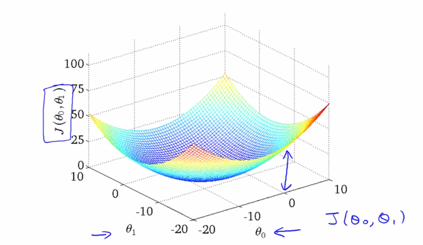
3D Parabola

• $J(\theta_0, \theta_1)$ as Z-Axis

• $\theta_0$ as X-Axis

• $\theta_1$ as Y-Axis

  

Two Feature ($x_1, x_2$) and Three Parameters ($\theta_0$, $\theta_1$, $\theta_2$)

h = $\theta_0 + \theta_1 x_1 + \theta_2 x_2

That lives in 4 dimensions impossible to visualize

J($\theta_0$, $\theta_1$, $\theta_2$) as W-Axis

• $\theta_0$ as X-Axis
• $\theta_1$ as Y-Axis
• $\theta_2$ as Z-Axis

---

Contour Figure ⛰️

Contour plot is seeing surface plot passing through a horizontal 2D clip plane

Each circle represents:

• All points that have the same height = Cost J(θ).

In the contour plot:

• X-axis → $\theta_0$
• Y-axis → $\theta_1$

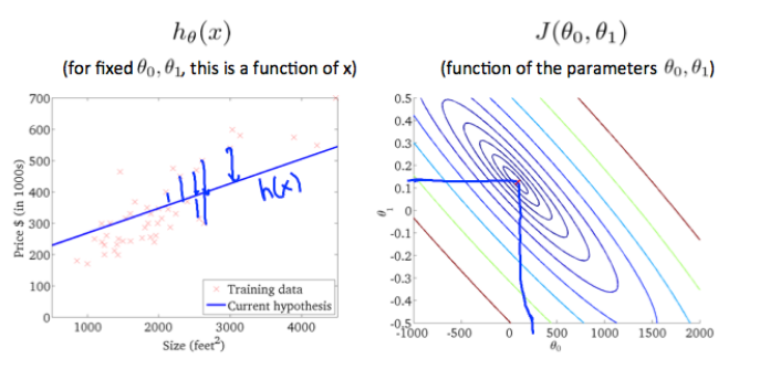
Why Contour Plot is Circular?

Contour Plot is Circular because Cost function is Convex.

• Circle represent all points that have the same height.
• Smaller circles → smaller cost
• Larger circles → larger cost

Gradient Descent Moves towards the center of the contour plot where cost is minimum.

• It moves perpendicular to the contour lines because that is the direction of steepest descent.

---

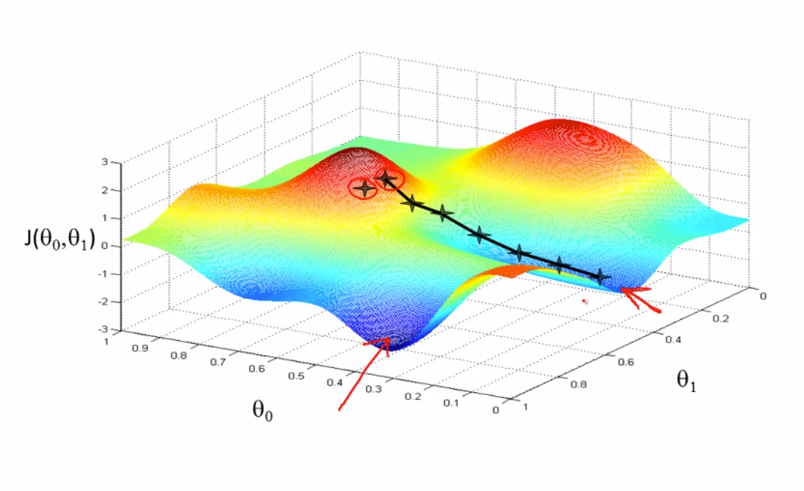
🎢 Gradient Descent

Gradient descent is an optimization algorithm used to minimize the cost function by iteratively moving towards the minimum.

That’s just a fancy name for:

Try numbers → see error → improve numbers → repeat.

Works like

• Start somewhere
• Just like going down from a hill.
• Look around and find local minima and keep on going down repeat till find optimal solution.
• Multiple minima can be found

Start somewhere → Take steps downhill → Reach minimum

Algorithm: Single Variant Linear Regression

For feature index j= 0, 1 repeat until convergence

$$\theta_j := \theta_j - \alpha \frac{1}{m} \sum_{i=1}^{m} \left( h_\theta(x^{(i)}) - y^{(i)} \right) x_j^{(i)}$$

For $j = 0,1$

• Simultaneous compute $\theta_0$, $\theta_1$ and store in temp values
• Simultaneous Update $\theta_0$, $\theta_1$

Where:

• $\alpha$ Learning Rate, How big steps we take down hill
• $_j$ is the parameter index
• $:=$ Assignment Operation eg a= a+1
• $=$ Truth Assertion eg a==a

This process is repeated until convergence.

Algo: Multivariate Linear Regression

Steps:

• For feature index j= 0,1,....n repeat until convergence

$$\theta_j := \theta_j - \alpha \frac{1}{m} \sum_{i=1}^{m} \left( h_\theta(x^{(i)}) - y^{(i)} \right) x_j^{(i)}$$

For $j = 0,1,2..n$

• Simultaneous Compute $\theta_0, \theta_1, .... \theta_n$ and store in temp values
• Simultaneous Update $\theta_0, \theta_1, .... \theta_n$

Final Hypothesis Function

$J(\theta) = \frac{1}{2m} \sum_{i=1}^{m} (h_\theta(x^{(i)}) - y^{(i)})^2$

Which is equivalent to: $J(\theta) = \frac{1}{2m} \sum_{i=1}^{m} (\theta^T x^{(i)} - y^{(i)})^2$

---

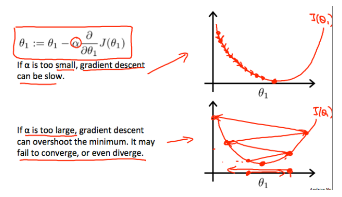
Learning Rate ($\alpha$)

Alpha defines rate of Learning

The update rule is:

$$\theta_j := \theta_j - \alpha \frac{\partial}{\partial \theta_j} J(\theta)$$

Or Simplified

$$\theta := \theta - \alpha \nabla J(\theta)$$

• Small $\alpha$ → slow learning
• Large $\alpha$ → overshooting the minimum
• Proper $\alpha$ → fast convergence

Deciding Learning Rate ($\alpha$)

Plot the cost function, $J(θ)$ over the number of iterations of gradient descent.

If $J(θ)$ decreases every iteration, then you are probably using a good learning rate.

• Smooth Steadily decreasing
• Flattening near minimum
• No wild jumps & no upward trend

       # Good Learning Rate
       
       |
       |\
       | \
       |  \
Cost   |   \
       |    \____
       |
       +----------------
       Iterations

If J(θ) continuously increases then you probably need to decrease $\alpha$.

• Reason: Large $\alpha$ causes overshooting the minimum, leading to divergence or oscillation.
• Fix: Reduce learning rate.

        |
        |      /
        |     /
Cost    |    /
        |   /
        |  /
        +----------------
        Iterations

If J(θ) decreases but very slowly, then you probably need to increase $\alpha$

• Reason: Small $\alpha$ causes slow convergence, taking many iterations to approach the minimum.
• Fix: Increase learning rate.

      Cost
        |
        |\
        | \
        |  \
        |   \
        |    \______
        +----------------
             Iterations

If J(θ) oscillates, then you probably need to reduce $\alpha$ and scale features.

• Reason:
  • Large $\alpha$ leading to oscillation around the minimum.
  • Features are on different scales,
• Fix: Reduce learning rate and apply feature scaling t

    Cost
    |
    |   /\   /\   /\
    |  /  \ /  \ /  \
    | /
    +----------------
    Iterations

Debugging Learning Rate ($\alpha$)

Behavior	Problem	Fix
Cost increases	α too large	Reduce α
Oscillates	α too large	Reduce α + scale
Very slow decrease	α too small	Increase α
No improvement	Features not scaled	Apply scaling

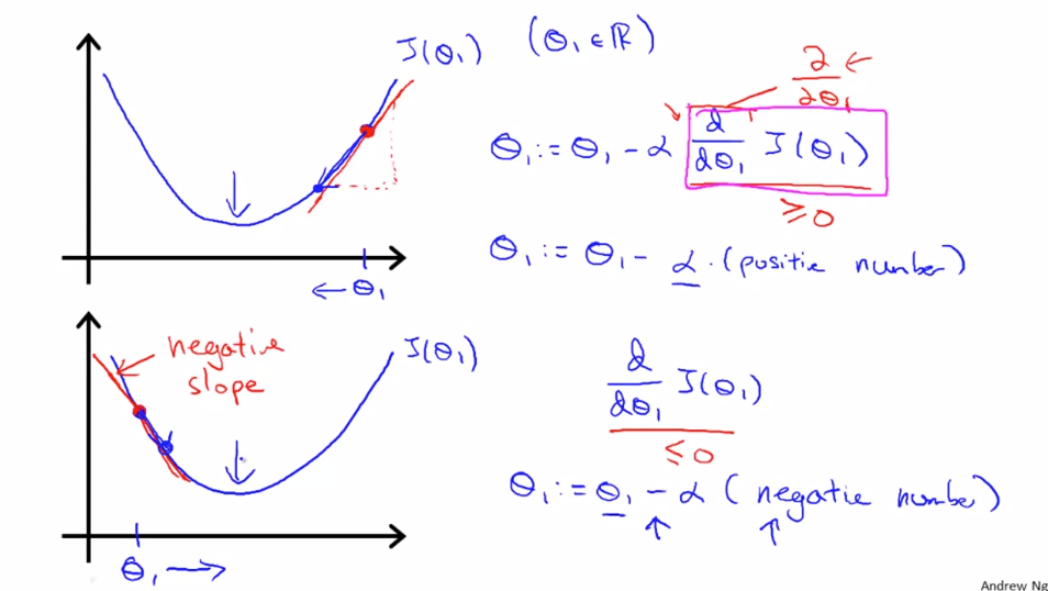
Derivative Term

Derivative terms defines rate of change of Cost function $J(\theta_1)$ wrt $\theta_1$

• At local minima Derivative Term is = 0.

$$\frac{\partial J(\theta)}{\partial \theta} = 0$$

• Derivative term automatically takes small step when it starts to converge towards local minimal. Having a fixed alpha helps

• Derivative term automatically converge $\theta_1$ towards its local minima from both +ve and -ve slopes:

  

---

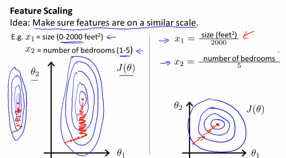
Feature Scaling

Feature scaling helps to make the cost function more circular, which allows gradient descent to converge faster.

• Make sure feature are on same scale otherwise contour will be skew elliptical.
• Try to get feature into $-1<= xi<= 1$
• Ideally should be withing range $-3<= xi<= 3$

Problem

Difference in scale of features can create skew ellipse in cost function.

• example:
  • Size of house (0-1000) vs Number of rooms (1-10)

A skew ellipse will have a long axis and a short axis.

• Gradient descent will oscillate across the long axis and take a long time to converge to the minimum.

📏 Solution

1. Min-Max Normalization

This is done by subtracting the minimum value of the feature and dividing by the range (max - min).

• Scale features to [0, 1]

$xi = \frac{xi - min(X)}{max(X) - min(X)}$

2. Mean Normalization:

This is done by subtracting the mean of the feature and dividing by the range (max - min).

• Scale features to have mean 0 and range [-3, 3]

$xi = \frac{xi - Avg(X)}{max(X) - min(X)}$

Alternatively

$xi = \frac{xi - \mu}{\sigma}$

Where:

• $\mu$ = mean of feature = Avg(X)
• $\sigma$ = standard deviation = max(X) - min(X)