Normal Equation in Linear Regression: Formula, Intuition, and Comparison with Gradient Descent

Normal Equation (Closed-Form Solution)

Instead of solving multiple iteration of gradient descent, Normal equation can get theta in one step

• Θ can be directly calculated where cost function is minimal using calculus in one step instead of iterating iterative optimization:

$$\theta = (X^T X)^{-1} X^T y$$

Advantages

• No learning rate required
• Direct computation

Limitations

• Computationally expensive for very large datasets
• Matrix inversion can be costly

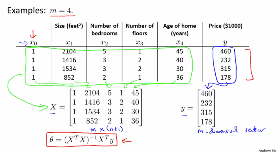
Steps:

• Construct design matrix X using feature columns and add 1 in first column
• Construct y vector using result values Y
• calculate:

Θ = (XTX)-1 XTy

Feature scaling is not required for Normal Equation method

Normal Equation vs Gradient Descent:

Feature	Gradient Descent	Normal Equation
Complexity	Complex need to debug alpha	Convenient & Simple to implement
Choose Learning Rate(α)	Required	No need
Feature Scaling	Required	No need
Iteration	Many Iteration Required	Not required
Feature Set>=million	Efficient if n is huge O(kn2)	Slow if n is huge, cost of inverse matrix is O(n3)
Complex Learning Algo	Can used for Complex learning algo	Not supported

---

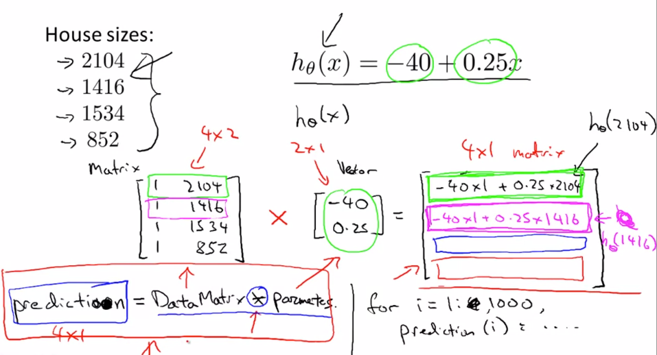
Faster single Hypothesis Prediction calculation given data set and Thetas **Much faster than nested for loops

Data Matrix * Parameter Vector = Prediction Vector

h(x) = Theta0 + Theta1x
[1 , x]*[Theta Vector] = [h(x)]

Usage:

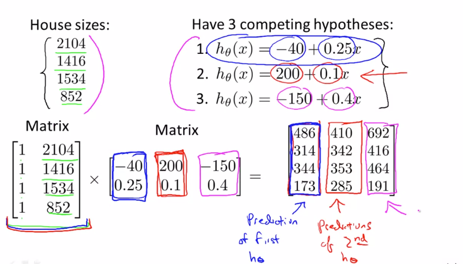
• Faster multiple Hypothesis Prediction calculation given data set and Thetas
• Much-much faster than nested for loops

Data Matrix * Parameter Matrix = Prediction Matrix

  given h(x) = Theta0 + Theta1x

  [1 , x]*[Theta Matrix] = [h(x)]