Normal Equation in Linear Regression

Normal Equation (Closed-Form Solution)

Instead of solving multiple iteration of gradient descent, Normal equation can get theta in one step

• Θ can be directly calculated where cost function is minimal using calculus in one step instead of iterating iterative optimization:

$$\theta = (X^T X)^{-1} X^T y$$

Advantages

• No learning rate required
• Direct computation

Limitations

• Computationally expensive for very large datasets
• Matrix inversion can be costly

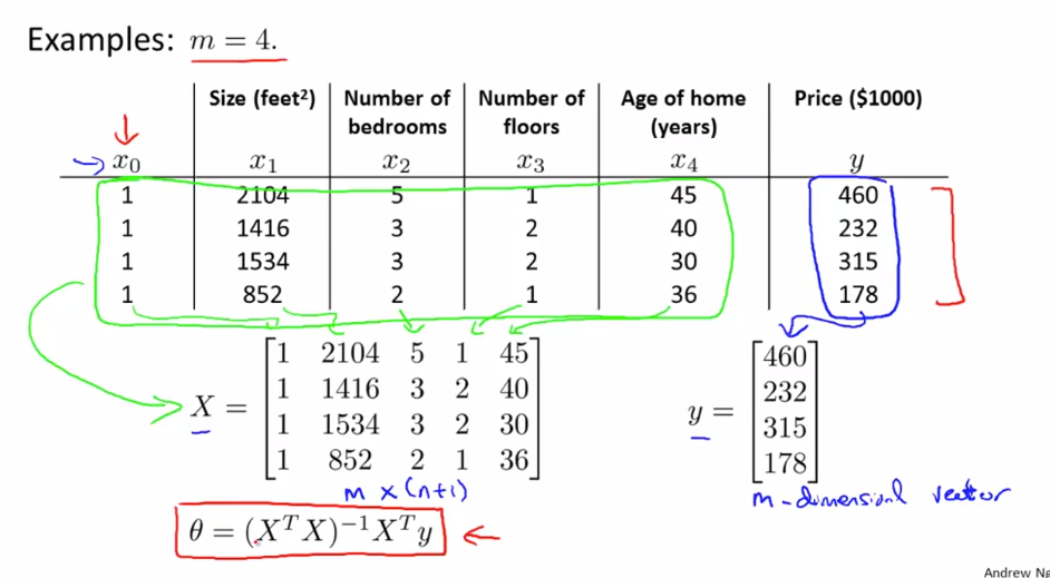
Steps:

• Construct design matrix X using feature columns and add 1 in first column
• Construct y vector using result values Y
• calculate:

Θ = (X^TX)^-1 X^Ty

Feature scaling is not required for Normal Equation method

Normal Equation vs Gradient Descent:

Feature	Gradient Descent	Normal Equation
Complexity	Complex need to debug alpha	Convenient & Simple to implement
Choose Learning Rate(α)	Required	No need
Feature Scaling	Required	No need
Iteration	Many Iteration Required	Not required
Feature Set>=million	Efficient if n is huge O(kn2)	Slow if n is huge, cost of inverse matrix is O(n3)
Complex Learning Algo	Can used for Complex learning algo	Not supported

---

Inverse Matrix(A^-1)

A' called inverse if

  A'.A = A'.A = I

Matrix without Inverse called Degenerate Matrix/ Singular/ Non Invertible

Cause for non invertible Matrix:

• Redundant feature: two feature related by a linear equation x2 = kx1 eg: size in feet and meter
• More feature than training set(m<=n)): delete some feature or use regularization

Octave method for inverting matrix:

• pinv(A) : Pseudo Inverse, calculates inverse even if matrix is non invertible
• inv(A) : Inverse