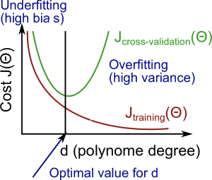
Bias-Variance Dilemma

Ideally, one wants to choose a model that both accurately captures the regularities in its training data, but also generalizes well to unseen data.

Bias

Error from erroneous assumptions in the learning algorithm.

• High bias can cause an algorithm to miss the relevant relations between features and target outputs (underfitting).

variance

Error from sensitivity to small fluctuations in the training set.

• High variance may result from an algorithm modeling the random noise in the training data (overfitting).

Bias vs Variance Summary

Concept	Meaning	Cause	Effect
High Bias	Model too simple	Too few features	Underfitting
High Variance	Model too complex	Too many features	Overfitting

Underfitting (High Bias)

Underfitting occurs when a model is too simple to capture the underlying pattern of the data, resulting in poor performance on both training and test data. If the real data has curvature, a straight line cannot capture it. This is called:

Cause:

• The model is too simple
• It fails to capture structure in the data

Problem:

• Poor training performance
• Poor Test performance

Overfitting (High Variance)

Overfitting happens when a model is too complex and starts fitting the training data perfectly, including noise, instead of capturing the real pattern.

• Model can bend heavily to pass through every training point.

Cause:

• The model is too complex
• It captures noise in the training data as if it were a true pattern

Problem:

• Low training error Good training performance but poor test performance
• This leads to poor performance on unseen data.
• Poor generalization to new data

Solutions

1. Reduce model complexity (e.g., use fewer features, simpler model)

• Reduce Number of Features: Manually select important features
• Use automated model selection methods
• Remove irrelevant variables

This simplifies the model.

2. Use regularization techniques (e.g., Lasso, Ridge)

• Instead of removing features, keep them all but reduce parameter sizes.

• Regularization adds a penalty term to the cost function to discourage complexity.

• Regularization helps prevent overfitting by keeping the model simpler.

• The regularization parameter λ controls the strength of the penalty. A larger λ means more regularization.

Lasso vs Ridge

Feature	Lasso (L1)	Ridge (L2)
Penalty	Sum of absolute values $\sum \| \theta_j\|$	Sum of squares $\sum \theta_j^2$
Effect	Can shrink some coefficients exactly to 0 → feature selection	Shrinks coefficients but rarely to 0
Use Case	Many irrelevant features	Prevent overfitting, keep all features

---

Instead of removing features, keep them all but reduce parameter sizes.

The idea:

• Large weights → complex model
• Small weights → smoother model

🔹 Lasso Regression (L1 Regularization)

Lasso: Cost = MSE + λ * sum(|θ|)

• Lasso (L1) can shrink some coefficients to zero, effectively performing feature selection.

In standard linear regression, the cost function is:

$$J(\theta) = \frac{1}{2m} \sum_{i=1}^{m} (h_\theta(x^{(i)}) - y^{(i)})^2$$

Lasso adds a penalty proportional to the sum of absolute values of the coefficients:

$$J(\theta) = \frac{1}{2m} \sum_{i=1}^{m} (h_\theta(x^{(i)}) - y^{(i)})^2 + \lambda \sum_{j=1}^{n} |\theta_j|$$

Where:

• $\lambda$ = regularization strength
• $|\theta_j|$ = absolute value of parameter $\theta_j$
• $\theta_0$ (bias) is usually not penalized

🏔️ Ridge Regression (L2 Regularization)

Ridge: Cost = MSE + λ * sum(θ^2)

• Ridge (L2) shrinks coefficients but does not set them to zero.

The standard linear regression cost function is:

$$J(\theta) = \frac{1}{2m} \sum_{i=1}^{m} (h_\theta(x^{(i)}) - y^{(i)})^2$$

Ridge adds a penalty proportional to the sum of squared coefficients:

$$J(\theta) = \frac{1}{2m} \sum_{i=1}^{m} (h_\theta(x^{(i)}) - y^{(i)})^2 + \lambda \sum_{j=1}^{n} \theta_j^2$$

Where:

• $\lambda$ = regularization strength
• $\theta_j$ = model parameters
• $\theta_0$ (bias) is usually not penalized

---