Multivariate Gaussian Distribution

The multivariate Gaussian distribution is an extension of the normal (Gaussian) distribution to multiple variables.

It is commonly used in:

• anomaly detection
• probabilistic modeling
• Gaussian mixture models
• Bayesian ML
• Kalman filters

Motivation

Suppose we are monitoring machines in a data center.

Features:

Feature	Meaning
$x_1$	CPU Load
$x_2$	Memory Usage

Most machines behave normally:

High CPU  ↔ High Memory
Low CPU   ↔ Low Memory

The features are correlated.

Problem with Basic Gaussian Anomaly Detection

Earlier anomaly detection assumed:

$$p(x) = p(x_1)p(x_2)$$

meaning:

• features are independent

Why This Fails

Suppose we observe:

CPU Load   = Very Low
Memory Use = Very High

Individually:

• CPU value looks normal
• Memory value looks normal

But together:

• this combination is strange

Visual Intuition

Normal data may lie along a diagonal trend:

Low CPU  → Low Memory
High CPU → High Memory

An anomalous point:

Low CPU + High Memory

lies far away from the normal pattern.

Basic Gaussian fails because it ignores feature correlation.

Solution: Multivariate Gaussian

Instead of modeling each feature separately:

$$p(x_1), p(x_2), ..., p(x_n)$$

we model:

$$p(x)$$

all together.

Multivariate Gaussian Formula

The probability density is:

$$p(x;\mu,\Sigma) = \frac{1}{ (2\pi)^{n/2} |\Sigma|^{1/2} } \exp \left( -\frac{1}{2} (x-\mu)^T \Sigma^{-1} (x-\mu) \right)$$

No need to memorize this formula.

Parameters

1. Mean Vector $(\mu)$

Represents the center of the distribution.

Example:

$$\mu = \begin{bmatrix} 0 \\ 0 \end{bmatrix}$$

means:

• centered at origin

2. Covariance Matrix $(\Sigma)$

An $(n \times n)$ matrix describing:

• variances
• correlations

Covariance Matrix Structure

For 2 features:

$$\Sigma = \begin{bmatrix} \sigma_1^2 & correlation \\ correlation & \sigma_2^2 \end{bmatrix}$$

1. Diagonal Entries

Represent variance of each feature.

Example:

$$\Sigma = \begin{bmatrix} 1 & 0 \\ 0 & 1 \end{bmatrix}$$

means:

• both features have equal variance
• no correlation

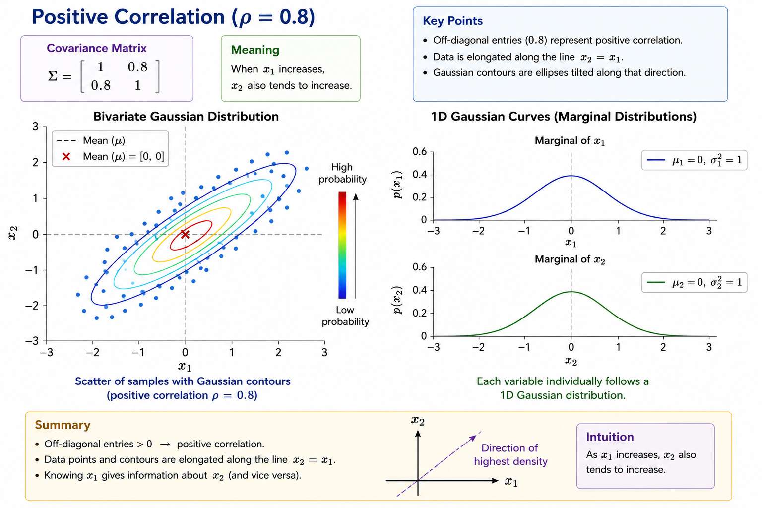
2. Off-Diagonal Entries

Represent correlation between features.

Positive Correlation

Example:

$$\Sigma = \begin{bmatrix} 1 & 0.8 \\ 0.8 & 1 \end{bmatrix}$$

Meaning:

When x1 increases
x2 also tends to increase

Probability mass lies near:

$$x_1 \approx x_2$$

Visual Shape

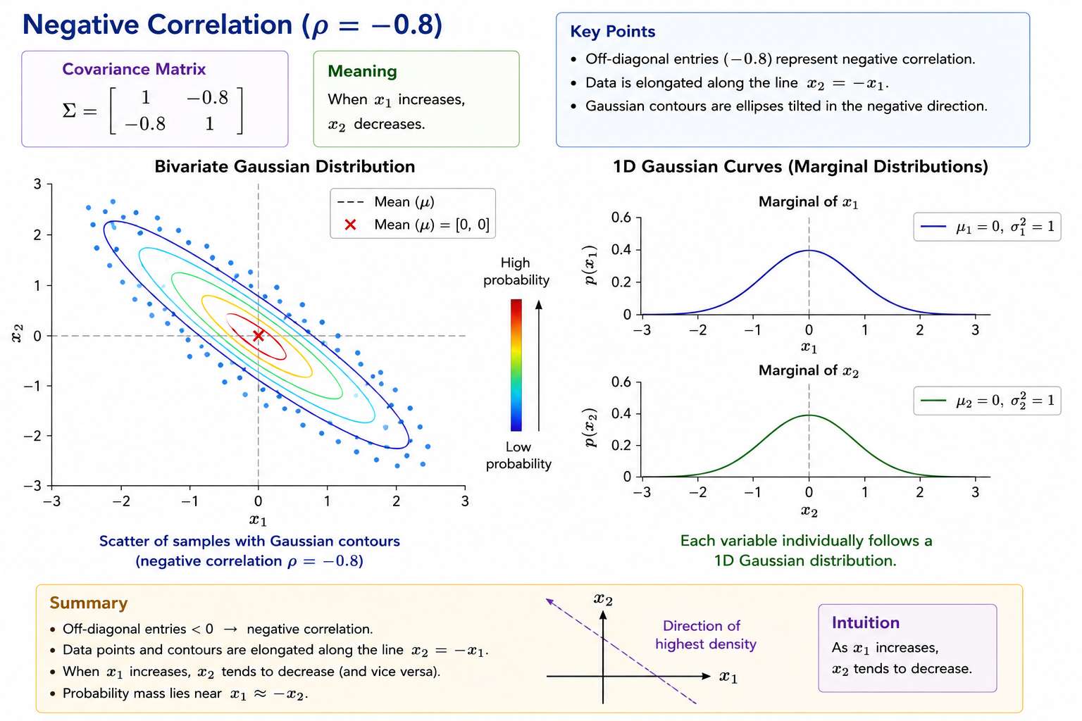
Negative Correlation

Example:

$$\Sigma = \begin{bmatrix} 1 & -0.8 \\ -0.8 & 1 \end{bmatrix}$$

Meaning:

When x1 increases
x2 decreases

Probability mass lies near:

$$x_1 \approx -x_2$$

Visual Shape

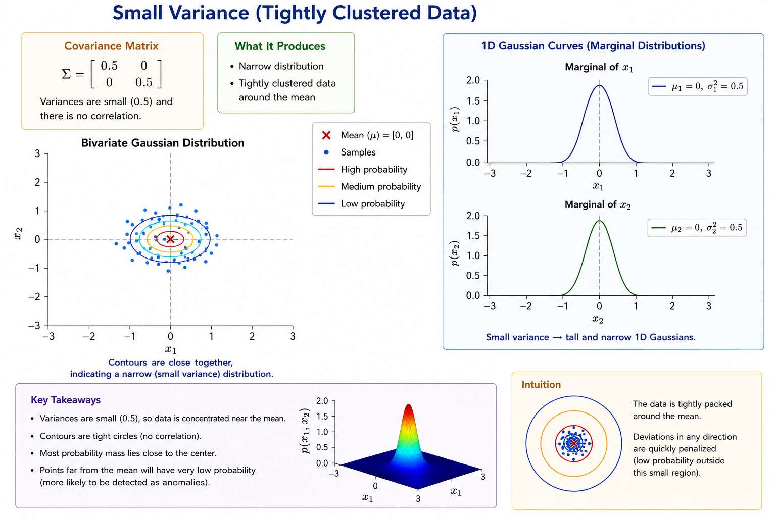
3. Effect of Variance

Small Variance

$$\Sigma = \begin{bmatrix} 0.5 & 0 \\ 0 & 0.5 \end{bmatrix}$$

Produces:

• narrow distribution
• tightly clustered data

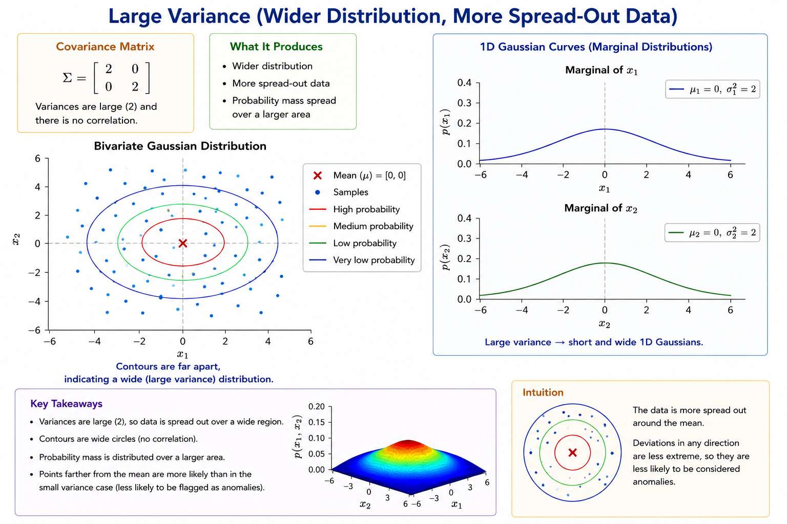
Large Variance

$$\Sigma = \begin{bmatrix} 2 & 0 \\ 0 & 2 \end{bmatrix}$$

Produces:

• wider distribution
• more spread-out data

Geometric Interpretation

Multivariate Gaussian creates:

Elliptical Probability Regions

High Probability
    ↓
   ****
 ********
**********
 ********
   ****

Points near center:

• high probability

Points far away:

• low probability

Anomaly Detection

Compute:

$$p(x)$$

If:

$$p(x) < \epsilon$$

then:

x is an anomaly

Why Multivariate Gaussian Is Better

Basic Gaussian:

• assumes features independent

Multivariate Gaussian:

• models correlations

This helps detect anomalies like:

Low CPU + High Memory

even if each feature individually looks normal.

Comparison

Method	Assumes Independence?	Captures Correlation?
Basic Gaussian	Yes	No
Multivariate Gaussian	No	Yes

---

Visual Comparison

Basic Gaussian

Circular contours

Assumes equal independent spread.

Multivariate Gaussian

Tilted elliptical contours

Captures relationships between variables.

Mean Shifts Distribution

Changing:

$$\mu$$

moves the center.

Example:

$$\mu = \begin{bmatrix} 1.5 \\ -0.5 \end{bmatrix}$$

shifts peak to:

x1 = 1.5
x2 = -0.5

Complete Anomaly Detection Pipeline

flowchart TD
    A[Collect Normal Data]
    --> B[Estimate μ and Σ]
    --> C[Compute p(x)]
    --> D[{p(x) < ε ?}]
    -->|Yes| E[Anomaly]
    -->|No| F[Normal Example]

Advantages

###aptures Correlations

Very important for real-world systems.

More Expressive

Can model:

• tilted distributions
• elongated regions
• correlated variables

Disadvantages

Needs more data.

Why?

Because covariance matrix has many parameters:

$$n \times n$$

For large (n):

• expensive
• harder to estimate reliably

Practical Rule

Use Basic Gaussian When

• features mostly independent
• small dataset
• high dimensionality

Use Multivariate Gaussian When

• features strongly correlated
• enough training data available

---