Anomaly Detection Using Gaussian Distribution

In this approach, we build an anomaly detection algorithm by modeling the probability of data using Gaussian distributions.

1. Model each feature using a Gaussian distribution.
2. Estimate $\mu$ and $\sigma^2$ from training data.
3. Compute $p(x)$ for new examples.
4. Flag examples where:

$$p(x) < \varepsilon$$

Low probability → likely anomaly.

---

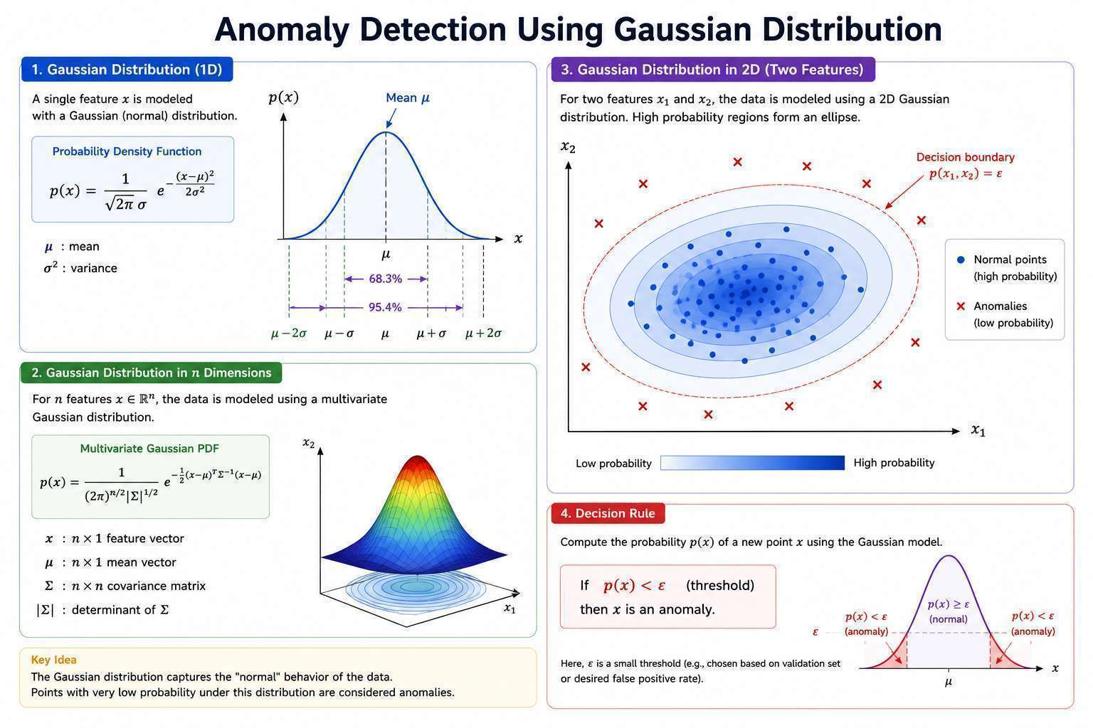
🔔 Understanding Gaussian Distribution

Probability Density Function

The Gaussian probability density function is:

$$p(x) = \frac{1}{\sqrt{2\pi}\sigma} e ^{ -\frac{(x-\mu)^2}{2\sigma^2}}$$

Where:

• $x$ = random variable in data set
• $\mu$ = mean : average of all data points
• $\sigma$ = standard deviation : how much data varies from the mean
• $\sigma^2$ = variance : square of standard deviation

Shape of the Gaussian Distribution

The Gaussian curve has the following properties:

• It is bell-shaped
• It is symmetric around the mean
• The total area under the curve equals 1

When plotted:

Any random variable $x$ follows a Gaussian distribution with:

$$x \sim \mathcal{N}(\mu, \sigma^2)$$

Where

The symbol $\sim$ means “is distributed as”.

$$x^{(1)}, x^{(2)}, ..., x^{(m)}$$

---

Effect of Parameters

The curve is fully defined by two parameters. So our goal is to estimate:

Normal case: μ = 0, σ = 1

This is the standard normal distribution.

• Centered at 0
• Moderate width

1. Mean (μ) ↔️

The average of all the data points

$$\mu = \frac{1}{m} \sum_{i=1}^{m} x^{(i)}$$

• Controls the center of the distribution.
• Changing μ shifts the curve left or right.

Example:

• If μ = 0 → centered at 0
• If μ = 3 → centered at 3

Effect of $\mu$ ↔️

$\mu$	$\sigma$	Shape of the Curve
0	1	Standard bell curve
3	1	Shifted to the right, same shape as standard curve
-2	1	Shifted to the left, same shape as standard curve

2. Standard Deviation ($\sigma^2$) ↕️

This measures how far the data points are from the mean.

It is the average squared deviation from the mean.

$$\sigma^2 = \frac{1}{m} \sum_{i=1}^{m} (x^{(i)} - \mu)^2$$

• Controls the width of the curve.
• Smaller $\sigma$ → narrower and taller curve
• Larger $\sigma$ → wider and flatter curve

Since total area must equal 1:

• If the curve gets wider → it becomes shorter
• If the curve gets narrower → it becomes taller

Effect of $\sigma$ ↕️

$\mu$	$\sigma$	Shape of the Curve
0	1	Standard bell curve
0	0.5	Narrower and taller curve
0	2	Wider and flatter curve

Note on 1/m vs 1/(m−1)

In statistics, you may sometimes see:

$$\frac{1}{m-1}$$

instead of:

$$\frac{1}{m}$$

In machine learning, we usually use 1/m. When the dataset is large, the difference is very small in practice.

---

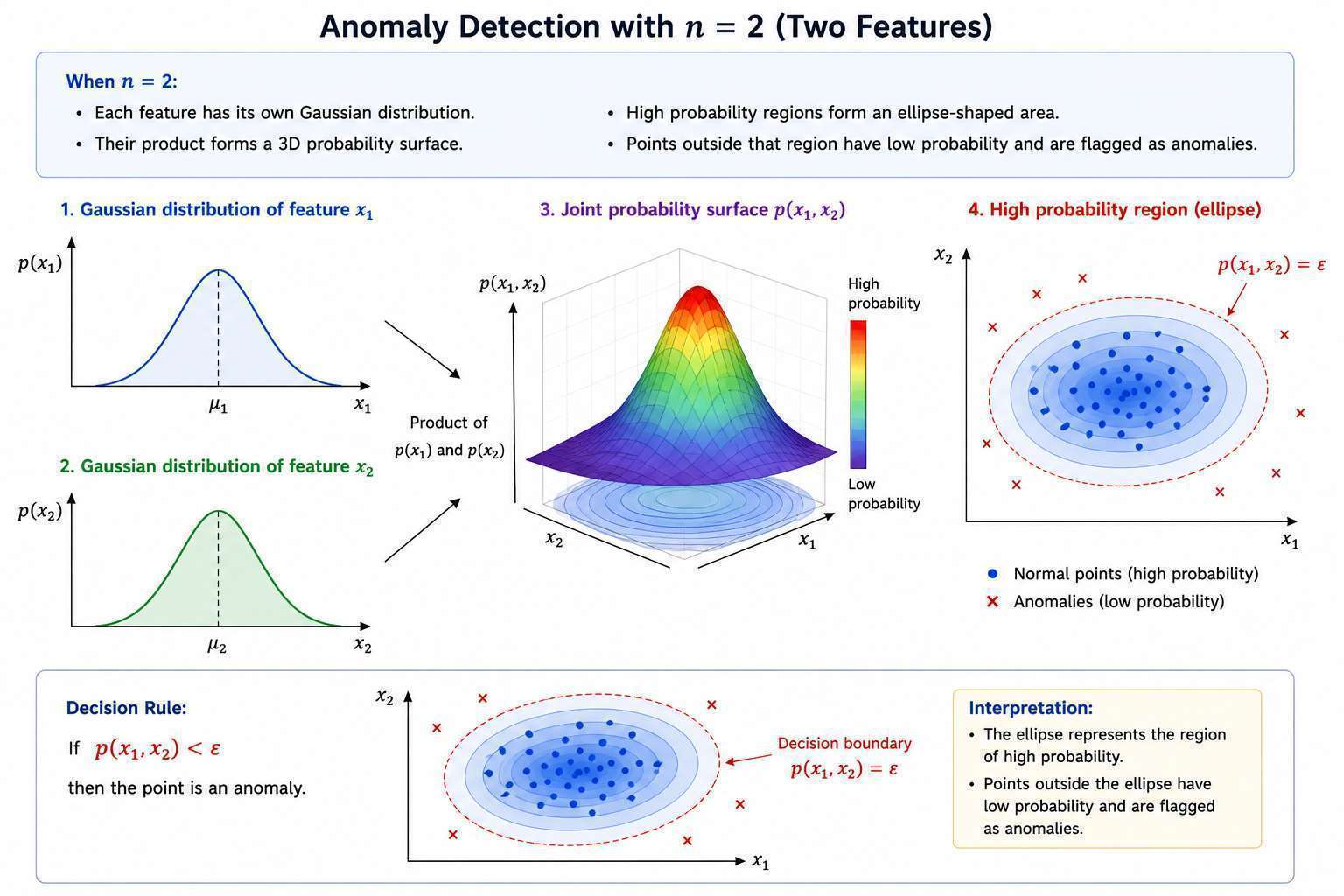
Intuition (2D Case)

When $n = 2$:

• Each feature has its own Gaussian distribution.
• Their product forms a 3D probability surface.
• High probability regions form an ellipse-shaped area.
• Points outside that region have low probability and are flagged as anomalies.

Problem Setup

We are given:

• An unlabeled training set of $m$ examples:

  $$x^{(1)}, x^{(2)}, \dots, x^{(m)}$$

• Each example is a feature vector in $\mathbb{R}^n$

Examples:

• Aircraft engine sensor data
• User behavior features
• System monitoring metrics

The goal is to determine whether a new example is normal or anomalous.

1. Training Phase 📚

1. Choose relevant features.
2. Compute $\mu_1, \dots, \mu_n$.
3. Compute $\sigma_1^2, \dots, \sigma_n^2$.

Modeling $p(x)$

We model the probability of a data point using Gaussian Distribution:

$$p(x) = p(x_1, x_2, \dots, x_n)$$ $$x \in \mathbb{R}^n$$

where $n$ is the number of features.

Each feature is modeled using a Gaussian distribution:

$$x_j \sim \mathcal{N}(\mu_j, \sigma_j^2)$$

The symbol $\sim$ means “is distributed as”.

This means the random variable $x$ follows a Gaussian distribution with:

• Mean $\mu_j$
• Variance $\sigma_j^2$

1. Parameter Estimation

Given training data, we estimate parameters.

Mean $\mu_j$

For each feature $j$:

$$\mu_j = \frac{1}{m} \sum_{i=1}^{m} x_j^{(i)}$$

This is the average value of feature $j$.

Variance $\sigma_j^2$

$$\sigma_j^2 = \frac{1}{m} \sum_{i=1}^{m} \left(x_j^{(i)} - \mu_j\right)^2$$

This measures how spread out the feature values are.

2. Density estimation 🌌

Compute Probability of Examples

Probabilities are multiplicative for independent features.

$p(x) = p(x_1, x_2, \dots, x_n)$

We assume the features are independent, so:

$$p(x) = \prod_{j=1}^{n} p(x_j)$$

Here, $\prod$ denotes a product (multiplication over a range).

$$p(x) = \prod_{j=1}^{n} p(x_j; \mu_j, \sigma_j^2)$$

Where each feature probability is:

$$p(x_j) = \frac{1}{\sqrt{2\pi}\sigma_j} \exp\left( -\frac{(x_j - \mu_j)^2}{2\sigma_j^2} \right)$$

Example

For a 2-feature example:

Temperature

• $x_1$ = 17.5

• $p(x_1) = 0.0738$

Vibration Intensity

• $x_2$ = 48
• $p(x_2) = 0.02288$

To find the overall probability of this example:

$$p(x) = p(x_1) \times p(x_2)$$

Therefore:

$p(x) = 0.0738 \times 0.02288$

$p(x) = 0.001688544$

$p(x) \approx 0.00169$

---

2. Making Predictions 🔎

Detection Phase

For a new example $x_{test}$:

Step 1: Compute probability

$$p(x_{test}) = \prod_{j=1}^{n} p(x_{test,j}; \mu_j, \sigma_j^2)$$

Step 2: Choose threshold $\varepsilon$

Decision Rule

Compare with $\varepsilon$.

$$\text{If } p(x_{test}) < \varepsilon \Rightarrow \text{Anomaly}$$ $$\text{If } p(x_{test}) \ge \varepsilon \Rightarrow \text{Normal}$$

Flag as anomaly if probability is low.

---

Key Takeaway

The multivariate Gaussian distribution models:

Feature Variance
+
Feature Correlation

which allows anomaly detection systems to detect unusual combinations of features, not just unusual individual values.