Graphics

Plotting

• Plots Y against X

---

Line Specification

Line Style

'-'    Solid line (default)
'--'   Dashed line
':'    Dotted line
'-.'   Dash-dot line

Marker Symbol

'.'    Point
'x'    Cross
'+'    Plus sign
'o'    Circle
'*'    Asterisk
'^'    Upward-pointing triangle
'v'    Downward-pointing triangle
'>'    Right-pointing triangle
'<'    Left-pointing triangle
's'    Square
'd'    Diamond
'p'    Five-pointed star (pentagram)
'h'    Six-pointed star (hexagram)

Color

r    Red
g    Green
b    Blue
c    Cyan
m    Magenta
y    Yellow
k    Black
w    White

---

Plotting Commands

plot(x, y)
plot(x, y, "r*")          % red asterisk, no line

hold on                    % plot on same axes as before
hold off                   % plot on different axes

clf                        % clear figure
close                      % close figure

figure(1); plot(x, y)     % save a named figure

subplot(n, m, o)          % divide plot into n×m grid, activate slot o
subplot(1, 2, 1)          % 1×2 grid, draw in first subplot

plot(Vector)              % auto-plot vector on Y axis
plot(x, y, "red--o", "LineWidth", 4)

Axis Limits

xlim([n, m])   % limit x range
ylim([n, m])   % limit y range

---

Plot Matrix

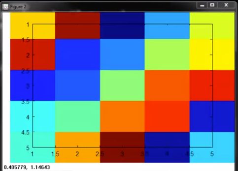
Color Plot

A = magic(5);
imagesc(A)

Result:

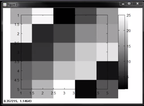
Grey Scale Plot

A = magic(5);
imagesc(A), colorbar, colormap grey

Result:

---

Labels & Legend

title('Title of Plot')
xlabel('X Axis Label')
ylabel('Y Axis Label')
legend('plot1', 'plot2')
axis([x1, x2, y1, y2])    % set axis range
grid on                    % enable grid

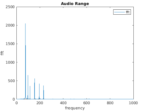
Example: FFT Plot

plot(f, yfft)
xlim([0, 1000])
title("Audio Range")
xlabel("Frequency")
ylabel("FFT")
legend("fft")

Result:

---

Export Figure

print -dpng "<image_name>.png"