🧱 Data Structures: Arrays, Stacks, Queues, Heaps, Hash Tables, Tries & Graphs
Data structures from the ground up — why arrays and linked lists trade off access vs insertion, real Java examples for arrays/lists/stacks/queues, a Binary Heap stored with no pointers at all, how a hash table actually resolves collisions, tries for prefix matching, graph representations, and a practical guide to choosing the right structure.
🧪 Testing 📖
🌲 Trees Deep Dive: BST, AVL Rotations, Red-Black Trees, B-Trees & B+ Trees
Data Structures
Every data structure is a tradeoff, never a free lunch
- an array gives you access by paying for it with insertion;
- a linked list flips that trade the other way.
There's no single "best" structure, only the one whose tradeoff matches what your code actually does most often: read a lot and rarely insert, or insert constantly and rarely search by index.
Visual Hierarchy
  Data Structures
  │
  ├── Linear
  │   ├── Array
  │   ├── Linked List
  │   ├── Stack
  │   └── Queue
  │
  └── Non-Linear
      ├── Trees
      │   ├── Binary Tree
      │   ├── Binary Search Tree ⚖
      │   ├── AVL Tree
      │   ├── Red-Black Tree
      │   ├── B-Tree
      │   └── Heap
      │
      ├── Graphs
      │   ├── Directed Graph
      │   ├── Undirected Graph
      │   ├── Weighted Graph
      │   └── DAG
      │
      ├── Trie
      └── Hash Table
Algorithmic Complexity
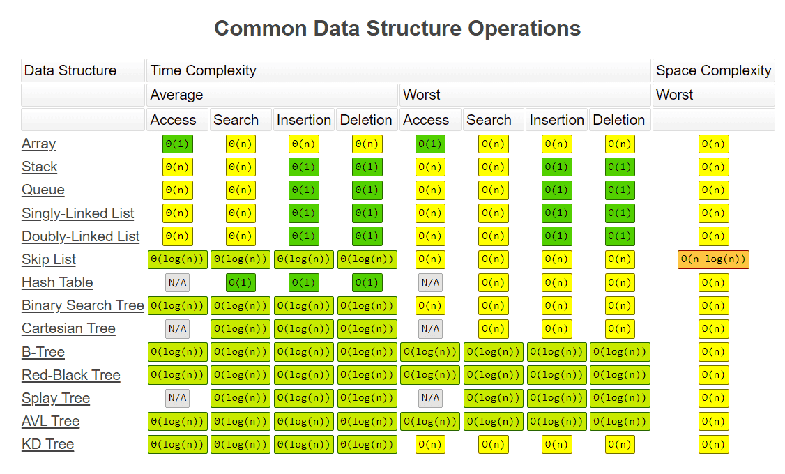
Every complexity number in the tables below — , , — comes from the same asymptotic (Big O) notation, derived and explained in depth in its own post:
👉 🔢 Algorithmic Complexity: Big O From First Principles
Linear Data Structures
| # | Data Structure | 📥 Access | ➕ Insertion | 🗑️ Deletion | Searching 🔍 |
|---|---|---|---|---|---|
| 1 | 🧮 Array | At 0 Index: | At 0 Index: | Linear: Binary Sorted: | |
| 2 | 🔗 Linked List | ||||
| 3 | 📚 Stack | ||||
| 4 | 🚶 Queue |
Array
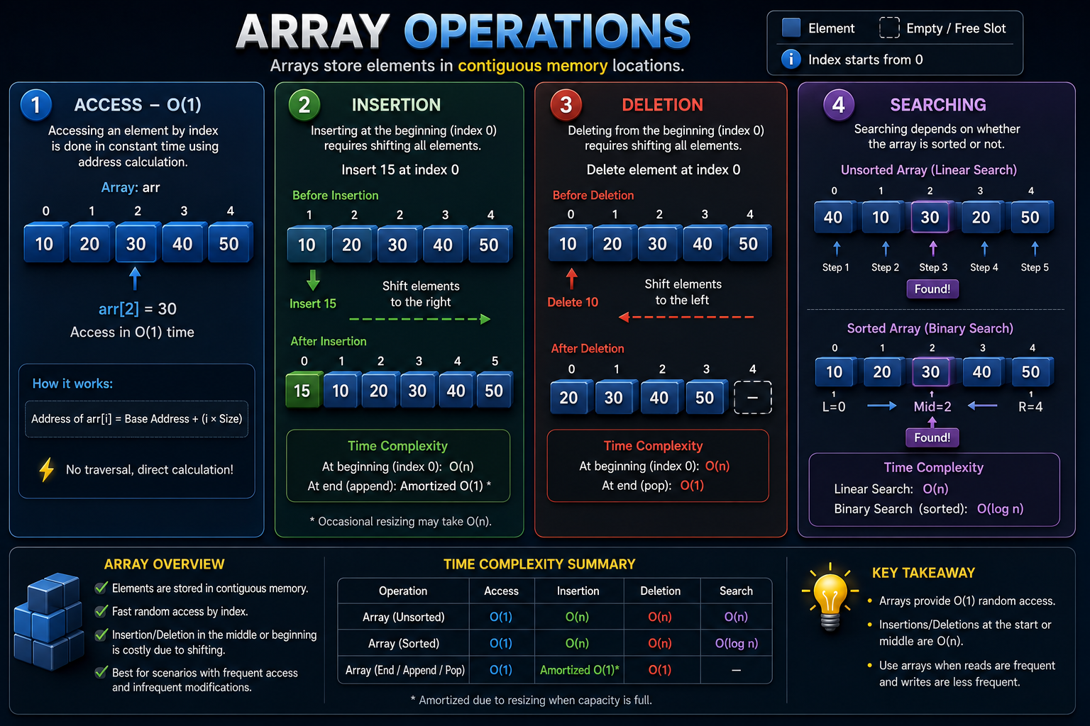
In an array's elements sit at a fixed memory offset from each other
Use an array when you know where you want to access data by index.
If fast random access is more important than frequent insertions or deletions, an array is usually the best choice.
flowchart LR
    N0["value 🔢 "] --> N1["value 🔢 "] --> N2["value 🔢 "]
Example:
int[] numbers = {10, 20, 30, 40};

System.out.println(numbers[2]); // 30

numbers[1] = 25;
✅ Array Advantages
- Constant-time random access
- Cache-friendly because elements are contiguous in memory
- Excellent iteration performance
- Minimal memory overhead compared to pointer-based structures
- Well suited for CPUs, SIMD instructions, and GPUs
❌ Array Limitations
- Inserting or deleting at the beginning or middle requires shifting elements
- Fixed size for static arrays (dynamic arrays may require resizing)
- Resizing a dynamic array may require allocating a new array and copying all elements
- Requires contiguous memory, which can be difficult for very large allocations
Array Properties
| Operation | Time Complexity |
|---|---|
| 📥 Access | |
| ➕ Insertion | Beginning: End (Append): Amortized |
| 🗑️ Deletion | Beginning: End (Pop): |
| 🔍 Searching | Linear: Binary (Sorted): |
-
Accessing ith element
arr[i]is one address calculation regardless of . -
Inserting/Deleting at index 0 means shifting every element after it one slot over
Linked List 🔗
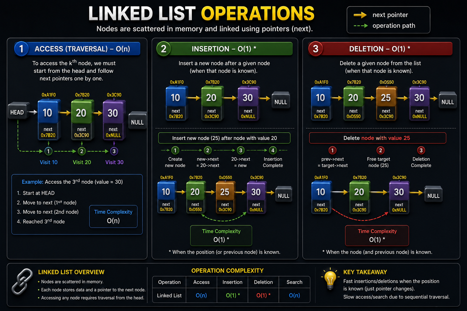
A linked list stores nodes anywhere in memory.
Each node contains the value and a pointer to the next node.
flowchart LR
    N0["Node<br/>value 🔢 | next 🔗"] --> N1["Node<br/>value 🔢 | next 🔗"] --> N2["Node<br/>value 🔢 | next 🔗"] --> Null["null"]
Use a linked list when your application frequently inserts or removes elements, especially in the middle of the collection, and fast random access is not required.
- LRU Cache
- Graph Representation
  import java.util.LinkedList;

  LinkedList<String> list = new LinkedList<>();

  list.add("A");
  list.add("B");
  list.addFirst("Start");
  list.addLast("End");

  list.removeFirst();
✅ Linked List Advantages
- Constant-time insertion and deletion once the node is known
- Dynamic size (grows and shrinks easily)
- No need for contiguous memory allocation
- Efficient for frequently changing collections
- Easy to split, merge, and reorder nodes by updating pointers
❌ Linked List Limitations
- Sequential access only (O(n))
- Extra memory overhead for storing pointers
- Poor cache locality due to scattered memory allocation
- Binary search is not practical because there's no direct indexing
Linked List Properties
| Operation | Time Complexity |
|---|---|
| 📥 Access | |
| ➕ Insert | Given node pointer: * Given Value |
| 🗑️ Delete | Given node pointer: * Given Value |
| 🔍 Search |
- Insertion and deletion are only if you already have a reference to the target node (or its predecessor in a singly linked list).
- Otherwise, finding the node takes .
Stacks and queues are abstract data types, not specific implementations. They can both be implemented using either an array or a linked list.
📚 STACK (LIFO)
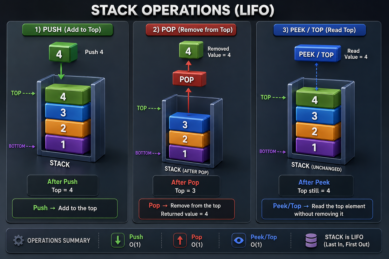
A stack follows the Last In, First Out (LIFO) principle.
A stack naturally models function calls, browser history, undo operations, and expression evaluation.
Every function call pushes a new stack frame, and every return pops one off.
flowchart TB
    Push["Push: Value 5 ➕"] --> E4
    Peek["Peek() 👀"] -.-> E4
    E4 --> Pop["Pop()🗑️"]

    subgraph Stack["Stack"]
        direction TB
        E4["Top: Value 4 🔢"]
        E3["Value 3 🔢"]
        E2["Value 2 🔢"]
        E1["Bottom: Value 1 🔢"]
        E4 --> E3
        E3 --> E2
        E2 --> E1
    end
- Push → Add to the top
- Pop → Remove from the top
- Peek/Top → Read the top element without removing it
Example
ArrayDeque is preferred over the legacy Stack class because it is faster and has a cleaner API.
  import java.util.ArrayDeque;
  import java.util.Deque;

  Deque<Integer> stack = new ArrayDeque<>();

  stack.push(10);
  stack.push(20);
  stack.push(30);

  System.out.println(stack.peek()); // 30
  System.out.println(stack.pop());  // 30
✅ Stack Advantages
- Constant-time push, pop, and peek operations
- Simple and efficient implementation
- Ideal for managing nested or recursive operations
- Requires access only to the top element
- Can be implemented using either an
array(fix size) or alinked list(dynamic)
❌ Stack Limitations
- Only the top element is directly accessible
- Searching for an arbitrary element requires traversing the stack (O(n))
- No random access to elements
- Not suitable when elements need to be processed in arbitrary order
- Array-based stacks have a fixed capacity unless dynamically resized
Stack Properties
| Operation | Time Complexity |
|---|---|
| 📥 Access | |
| ➕ Push | |
| 🗑️ Pop | |
| 👀 Peek (Top) | |
| 🔍 Search |
🚶 Queue (FIFO)
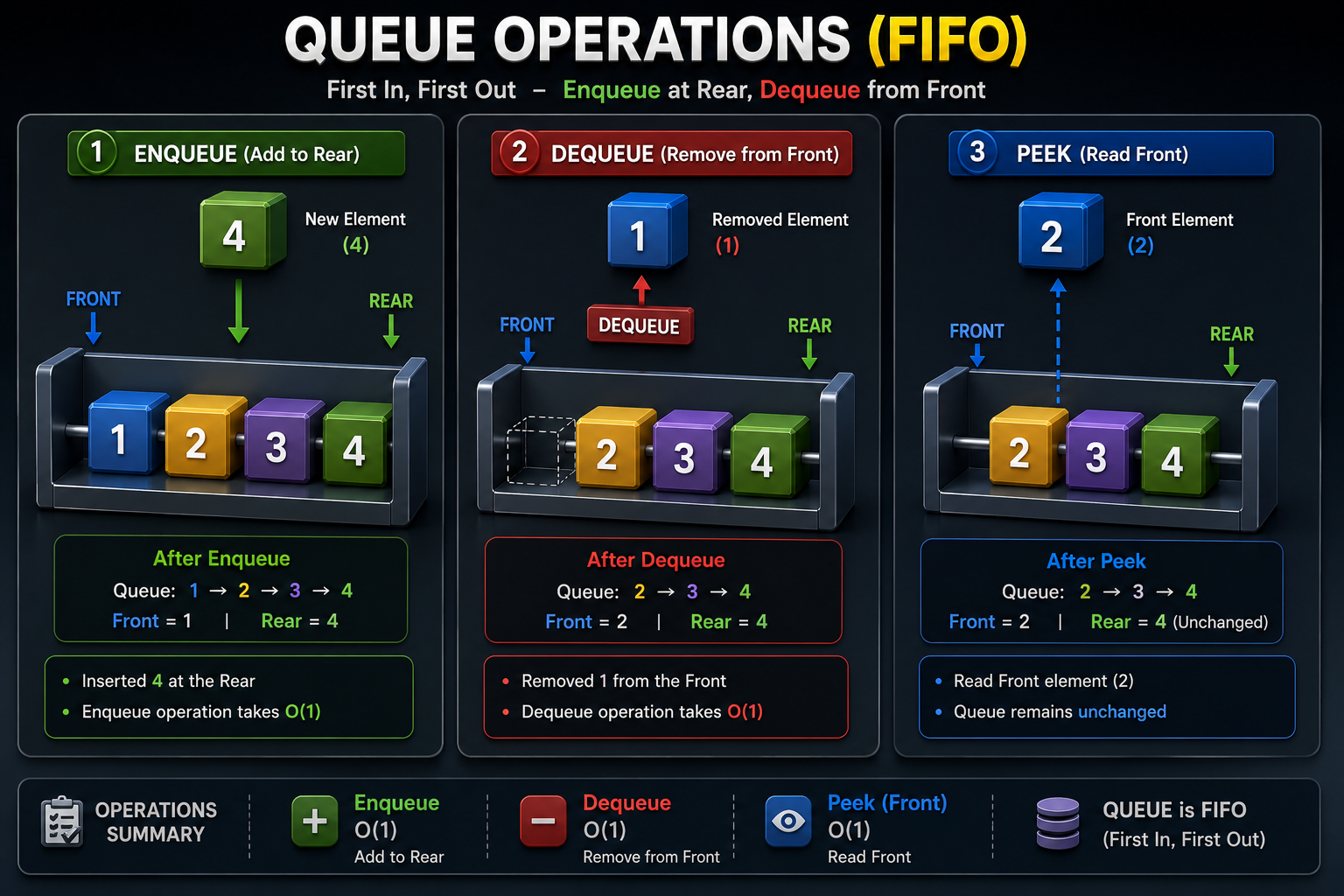
A queue follows the FIFO (First In, First Out) principle.
A queue models work that must be processed in arrival order, such as print queues, task schedulers, message brokers, and the frontier used in Breadth-First Search (BFS).
Elements are added at the rear (enqueue) and removed from the front (dequeue).
  flowchart TD
    subgraph Queue["Queue"]
        direction LR
        E1["Front: Value 1 🔢"]
        E1 --> E2["Value 2 🔢"]
        E2 --> E3["Rear: Value 3 🔢"]

    end

    Dequeue["Dequeue() 🗑️"] --> E1
    Peek["Peek() 👀"] -.-> E1
    Enqueue["Enqueue(4) ➕"] --> E3
- Enqueue → Add at the rear
- Peek → Read the front element
- Dequeue → Remove from the front
Example:
import java.util.ArrayDeque;
import java.util.Queue;

Queue<String> queue = new ArrayDeque<>();

queue.offer("A");
queue.offer("B");
queue.offer("C");

System.out.println(queue.peek()); // A
System.out.println(queue.poll()); // A
✅ Queue Advantages
- Constant-time
enqueue,dequeue, andpeekoperations - Processes elements in the exact order they arrive (FIFO)
- Fair scheduling for requests and tasks
- Efficient for producer-consumer and streaming workloads
- Can be implemented using either an array (circular queue) or a linked list
❌ Queue Limitations
- Only the front element is directly accessible
- Searching for an arbitrary element requires sequential traversal
- No random access by index
- Not suitable when the most recently added element should be processed first (use a stack instead)
- Array-based queues require a circular buffer or resizing to efficiently reuse freed space
Queue Properties
| Operation | Time Complexity |
|---|---|
| 📥 Access | |
| ➕ Enqueue | |
| 🗑️ Dequeue | |
| 👀 Peek (Front) | |
| 🔍 Search |
A Blocking Queue is a thread-safe queue designed for producer-consumer scenarios. Unlike a normal queue, operations can wait (block) until the queue is in the required state.
- Producer waits if the queue is full.
- Consumer waits if the queue is empty.
🌲 Non-Linear Data Structures
The tree family gets a full deep dive of its own — BST/AVL/Red-Black internals, all four AVL rotation cases, B-Trees/B+ Trees for database indexing, plus hash tables and tries:
👉 🌲 Trees Deep Dive: BST, AVL Rotations, Red-Black Trees, B-Trees & B+ Trees
⛰️ Binary Heap (Priority Queue)
A heap is a complete binary tree with a heap-order property: in a min-heap every parent ≤ its children ( max-heap: ≥). The smallest (or largest) element is always the root.
flowchart TB
    R["1 (min)"] --> A["3"]
    R["1 (min)"] --> B["2"]
    A["3"] --> C["7"]
    A["3"] --> D["5"]
    B["2"] --> E["4"]
Because it's complete, a heap is stored in a plain array with no pointers at all — for the node at index i,
children live at 2i+1 and 2i+2, parent at (i-1)/2. Index arithmetic replaces pointer chasing entirely.
- Peek (min/max) → read the root,
- Insert → append at the end, then sift up,
- Extract → swap root with last, remove, sift down,
- Search for an arbitrary value → ; a heap orders parent–child, not siblings, so there's no way to prune
Two interview gotchas worth banking: building a heap from an array is with Floyd's bottom-up method ( not — that's the naive insert-one-at-a-time build), and heaps power heapsort, Dijkstra's frontier, and top-k selection.
#️⃣ Hash Table & 🔤 Trie
Both get a full deep dive — collision resolution (chaining, linear/quadratic probing, double hashing), load factor and rehashing, and the Trie node structure with real diagrams — inside the Trees post above, right next to the tree structures they're most often compared against.
🕸️ Graph
Graphs get their own dedicated post — adjacency list vs matrix, and why BFS/DFS traversal cost is the floor every graph algorithm builds on:
👉 🕸️ Graph Data Structures: Adjacency List vs Matrix, BFS & DFS
Other Advanced Structures
| # | Data Structure | Access | Insertion | Deletion | Searching | Space |
|---|---|---|---|---|---|---|
| 1️⃣ | 📏 Segment Tree | ⚡ | ⚡ | ⚡ | ⚡ | 💾 |
| 2️⃣ | 🧬 Suffix Tree | ⚡ | ⚡ | ⚡ | ⚡ | 💾 |
A Segment Tree answers range queries (sum/min/max over [l, r]) in by precomputing partial results over
segments, updating in when a single element changes. A Suffix Tree indexes every suffix of a string,
enabling substring search in (the pattern length) regardless of how long the original text is — the same
-independent-of-corpus-size idea a trie applies to a word list, applied instead to every substring of one string.
How to Choose a Data Structure
| If you need to... | Use |
|---|---|
| Access elements by index constantly, rarely insert in the middle | Array |
| Insert/delete constantly at a known position, access by index rarely | Linked List |
| Process most-recent-first (undo, call stack, DFS) | Stack |
| Process first-in-first-out (task queue, BFS) | Queue |
| Look up by key with no ordering requirement | Hash Table |
| Look up by key and keep everything sorted / do range queries | Balanced BST (AVL / Red-Black) |
| Repeatedly grab the min/max element | Binary Heap (priority queue) |
| Store data on disk, minimize disk seeks | B-Tree (what most databases index with) |
| Autocomplete / prefix matching over strings | Trie |
| Model relationships/connections (sparse) | Graph — adjacency list |
| Model relationships/connections (dense, need edge checks) | Graph — adjacency matrix |
Key Takeaways
| Concept | Summary |
|---|---|
| Array vs Linked List | access vs insert — the tradeoff comes from contiguous memory vs scattered nodes with pointers |
| Stack / Queue | Both get operations by only ever touching one end (stack) or both ends (queue), never the middle |
| Binary Heap | Complete tree stored as a flat array — 2i+1/2i+2/(i-1)/2 index arithmetic replaces pointers; building from an array is , not |
| Hash Table & Trie | Deep dives live in the Trees post — collision handling, load factor, and the trie node structure |
| Graph | No single Big O — adjacency list ( space) wins for sparse graphs, matrix ( space, edge check) wins for dense ones; full post above |
| Segment / Suffix Tree | Specialized trees for range queries and substring search, both trading preprocessing time for fast repeated queries |
Every row in these tables is really answering the same question from a different angle: what did this structure choose to make fast, and what did it accept as slow in exchange? Knowing the tradeoff — not just memorizing the Big O column — is what lets you pick correctly for a problem the table never explicitly listed.
Related Posts
- 🌲 Trees Deep Dive — BST, AVL rotations, Red-Black Trees, B-Trees, hash tables, and tries
- 🕸️ Graph Data Structures — adjacency list vs matrix, BFS and DFS
- 🔢 Algorithmic Complexity — the Big O notation used throughout this post
- 🔎 Searching Algorithms — best/average/worst case complexity for linear, binary, and hashing-based search
- ⚡ Sorting Algorithms — complexity and stability comparison across the major sorting algorithms
- 🗄️ Database Comparison — how these structures show up as the storage engine underneath key-value, document, and relational databases