🔢 Algorithmic Complexity: Big O From First Principles
Asymptotic notation from the ground up — deriving Big O from a growth formula, a real timing table showing what each complexity class actually costs at n = 1,000,000, and every major growth order (constant, logarithmic, linearithmic, polynomial, exponential, factorial) with real code examples.
🕸️ Graph Data Structures: Adjacency List vs Matrix, BFS & DFS
🔎 Searching Algorithm Complexity 📖
🔢 Algorithmic Complexity
Asymptotic Notations
Measures the order of growth of an algorithm with respect to the number of inputs .
- Also called as Landau Notation (Edmund Landau)
| Notation | Bound | Common Usage |
|---|---|---|
| Big O | Upper Bound | Worst-case complexity |
| Little o | Upper Strict Bound | Mathematical analysis to show one function grows strictly slower than another |
| Big | Lower Bound | Best-case or guaranteed lower bound |
| Little ω | Lower Strict Bound | Mathematical analysis to show one function grows strictly faster than another |
| Big | Average Bound | Exact asymptotic complexity when both upper and lower bounds match |
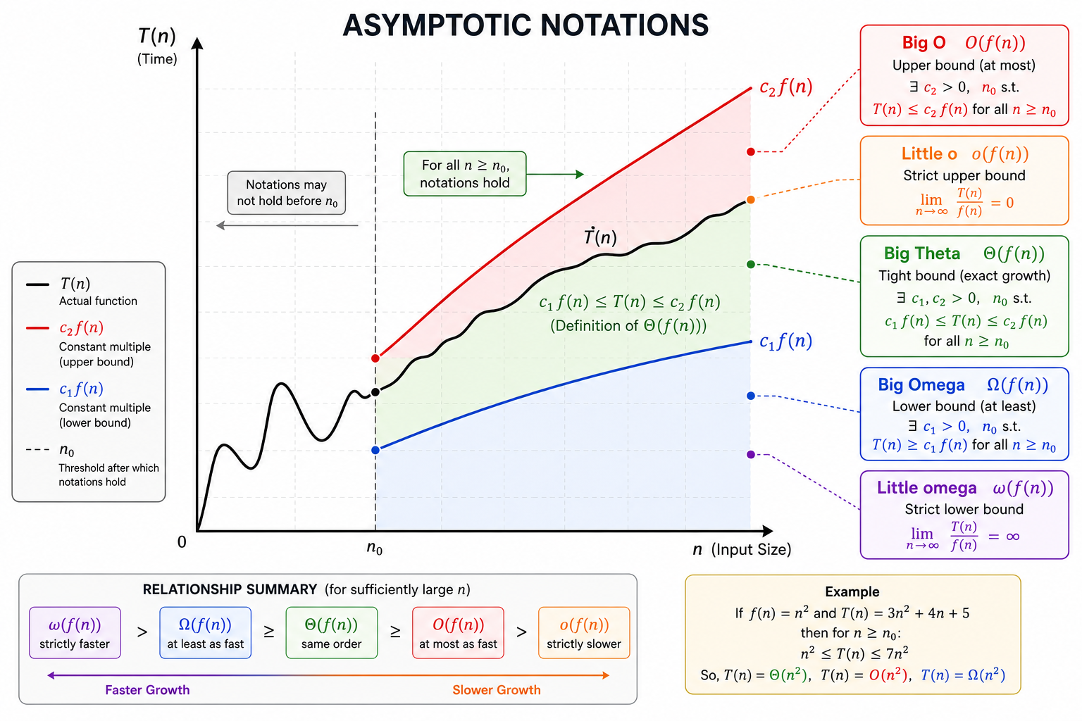
Example:
| Notation | Result | Meaning |
|---|---|---|
| Big | The function grows no faster than | |
| Little | The function grows strictly slower than | |
| Big | The function grows at least as fast as | |
| Little | The function grows strictly faster than | |
| Big | The function grows exactly like asymptotically. |
Big
Represents the worst-case scenario, where the loop runs till the last element.
- Fastest growing expression determine over all complexity.
- Remove Constant & Remove non-dominant terms
Example.
| Complexity | Operations (n = 1,000,000) | Approx. Time* |
|---|---|---|
| 1 | 1 ns | |
| ≈ 20 | 20 ns | |
| ≈ 400 | 400 ns (0.4 μs) | |
| 1,000 | 1 μs | |
| 1,000,000 | 1 ms | |
| ≈ 20,000,000 | 20 ms | |
| 1,000,000,000,000 | ≈ 16.7 minutes | |
| ≈ 31.7 years |
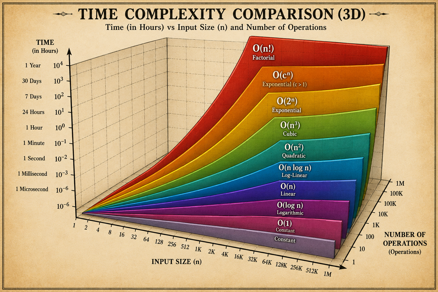
Commonly used big O notation
1. Constant time : -
Amount of work does not grow as the input size grows Fastest,
Independent of
- Single R/W
- Stack
push(),pop(),peek() - Hash table lookup (average case)
- Executes the same number of operations regardless of input size
2. Logarithmic : -
An algorithm has logarithmic time complexity when it reduces the problem size by a constant factor in each step, rather than processing every element.
Divide the input by a constant factor (usually 2) each iteration
Common in searching and tree-based algorithms
- Binary Search
- Divide & conquer
Example:
let n = 1024;

while (n > 1) {
  console.log(n);
  n = Math.floor(n / 2);
}
3. Poly Logarithmic :
If an algorithm performs a logarithmic amount of work multiple times, or has nested logarithmic operations, it often has polylogarithmic complexity
It grows slower than linear O(n) but faster than logarithmic .
Example:
let n = 1024;

for (let i = n; i > 1; i = Math.floor(i / 2)) {
for (let j = n; j > 1; j = Math.floor(j / 2)) {
  console.log(i, j);
}
}
1. Polynomial :
nested loops iterating over elements
Polynomial-time algorithms are generally considered efficient (or tractable) in computer science, especially compared to exponential and factorial algorithms.
| Name | Complexity |
|---|---|
| Linear | |
| Quadratic | |
| Cubic | |
| Quartic | |
| Quintic | |
| General Polynomial |
1.1 Linear : -
Grows proportionally to input size
- A single Loop iterating over n elements
- As number of elements grow time grows
1.2 Linearithmic :
Performs logarithmic work for each of the n elements, or repeatedly divides the problem and then performs linear work during each level of recursion.
Note: not strictly polynomial, but slots in here by growth rate
Faster than quadratic but slower than
Combines linear and logarithmic growth
Typical of efficient sorting algorithms
- Merge Sort
- Heap Sort
- Average-case Quick Sort
- Building a balanced Binary Search Tree
- Fast Fourier Transform (FFT)
Example:
let n = 1024;

for (let i = 0; i < n; i++) {                      // O(n)
  for (let j = n; j > 1; j = Math.floor(j / 2)) {  // O(log n)
    console.log(i, j);
  }
}
1.3. Quadratic :
Performs operations for each of the elements.
Typical of sorting algorithms
- Bubble Sort: O(n2)
- Selection Sort: O(n2)
Two nested linear loops:
Example:
let n = 1024;

for (let i = 0; i < n; i++) {      // O(n)
  for (let j = 0; j < n; j++) {    // O(n)
    console.log(i, j);
  }
}
1.4. Cubic :
Performs operations for each of the operations, typically due to three nested loops.
Three nested linear loops
- Naive matrix multiplication
- Floyd-Warshall shortest path algorithm
- Comparing every triplet of elements
- Brute-force solutions involving three independent variables
Example:
  let n = 100;

  for (let i = 0; i < n; i++) {          // O(n)
    for (let j = 0; j < n; j++) {        // O(n)
      for (let k = 0; k < n; k++) {      // O(n)
        console.log(i, j, k);
      }
    }
  }
2. Exponential :
For each element run nested loops
- Running time doubles, triples, or generally multiplies by a constant with each additional input
- Typically caused by recursive branching
- Becomes impractical even for moderate input sizes
If each recursive call branches into a constant number of new recursive calls, the algorithm usually has exponential time complexity, .
Example:
function solve(n) {
  if (n === 0) return;

  solve(n - 1);
  solve(n - 1);
}

solve(5);
grows faster than .
If grows faster than then it is called superpolynomial, and
in that case is called subexponential.
3. Factorial :
explores every possible ordering (permutation) of the input elements.
- Generating all permutations
- Brute-force Traveling Salesman Problem (TSP)
- Brute-force scheduling and assignment problems
- Exhaustive search over all possible orderings
Factorial growth is even faster than exponential growth. It becomes impractical for surprisingly small values of n.
Example;
function permute(arr, start = 0) {
  if (start === arr.length) {
    console.log(arr.join(" "));
    return;
  }

  for (let i = start; i < arr.length; i++) {
    [arr[start], arr[i]] = [arr[i], arr[start]];

    permute(arr, start + 1);

    [arr[start], arr[i]] = [arr[i], arr[start]];
  }
}

permute([1, 2, 3]);
If an algorithm has factorial complexity,
- first ask whether it's recomputing the same work or exploring impossible solutions.
- Memoization, dynamic programming, and pruning are the most common ways to reduce O(n!) to a much more practical complexity.
Related Posts
- 🧱 Data Structures — the structures whose Access/Insertion/Deletion/Search columns use this exact Big O notation
- 🔎 Searching Algorithms — Binary Search's is the logarithmic case worked through here
- ⚡ Sorting Algorithms — Merge Sort/Quick Sort's is the linearithmic case worked through here