Understanding U-Net

Deep learning has transformed computer vision, enabling machines to recognize objects, classify images, and understand scenes with remarkable accuracy. However, many real-world applications require more than classification. They require understanding where objects are located at the pixel level.

This task is known as image segmentation, and one of the most influential architectures for solving it is U-Net.

Originally developed for biomedical image segmentation, U-Net has become a cornerstone of modern computer vision and has even influenced the architectures used in today's diffusion-based image generation models.

In this article, we'll explore how U-Net works, why it became so successful, and how it continues to power cutting-edge AI systems.

What Is U-Net?

U-Net is a convolutional neural network (CNN) architecture designed for semantic segmentation.

Unlike image classification models that output a single label, U-Net predicts a class for every pixel in an image.

Example: Tumor Segmentation

Input:

Brain MRI Scan

Ground Truth:

Tumor Region

Output:

Predicted Tumor Mask

The network learns:

$$f(X)= Y$$

where:

• $X$ = MRI image
• $Y$ = segmentation mask

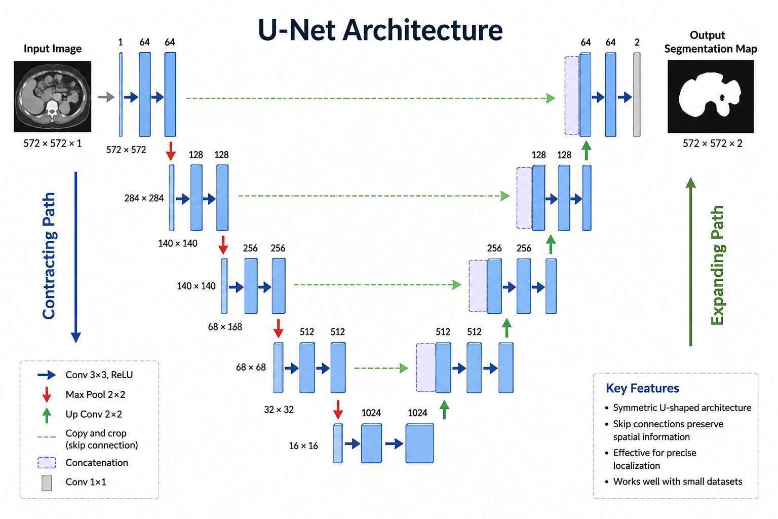
The architecture gets its name from its characteristic U-shaped structure.

graph TD

    A[Input Image 🖼️]

    A --> B[Encoder 📟]

   B --> C[Bottleneck 🚧]

    C --> D[Decoder 📟]

    D --> E[Segmentation Mask 🧩]

    B -. Skip Connections ⏭️ .-> D

Illustration of U-Net Working

The network consists of:

• Encoder (Contracting Path)
• Bottleneck
• Decoder (Expanding Path)
• Skip Connections

The left side compresses information.

The right side reconstructs information.

Together they form a U shape.

---

Why Image Segmentation Is Challenging

Consider a medical image:

MRI Scan

Traditional image classification answers:

Tumor Present

But doctors need:

Where is the tumor?

Segmentation provides this information by classifying every pixel.

Example:

Background = 0
Tumor = 1

Result:

Pixel-Level Prediction

This requires preserving spatial information throughout the network.

---

U-Net Architecture Breakdown

1. Encoder: The Contracting Path 📟

The encoder extracts increasingly abstract features.

Example progression:

graph TD

    Image[Input Image 🖼️]
    Edges[Edges 📐]
    Textures[Textures 🎨]
    Shapes[Shapes 🔺]
    Objects[Objects 🏥]

    Image --> Edges
    Edges --> Textures
    Textures --> Shapes
    Shapes --> Objects

Each encoder block typically contains:

• Convolution
• ReLU Activation
• Convolution
• Max Pooling

As the network moves deeper:

• Spatial resolution decreases
• Feature richness increases

Convolution Operations

The core operation is convolution.

Given:

$$X$$

as the input image and

$$K$$

as the kernel,

the output feature map becomes:

$$Y(i,j) = \sum_m \sum_n X(i-m,j-n)K(m,n)$$

This operation allows the network to detect:

• Edges
• Corners
• Textures
• Patterns

at different levels of abstraction.

As the network goes deeper:

• Resolution decreases
• Feature richness increases

---

2. Bottleneck Layer 🚧

At the center of the network lies the bottleneck.

graph TD

    Encoder[Encoder 📟]
    Bottleneck[Bottleneck 🚧]
    Decoder[Decoder 📟]

    Encoder
    Encoder --> Bottleneck
    Bottleneck --> Decoder

This layer contains the most compressed representation of the image.

It captures high-level semantic information while sacrificing spatial detail.

---

3. Decoder: The Expanding Path 📟

The decoder reconstructs the image.

• Its goal is to recover details lost during compression.
• The decoder reconstructs spatial information.

Process:

graph TD

    CompressedFeatures[Compressed Features 📦]
    Upsampling[Upsampling 📤]
    FeatureReconstruction[Feature Reconstruction ✨]
    PixelPrediction[Pixel Prediction 🪄]

    CompressedFeatures
    CompressedFeatures --> Upsampling
    Upsampling --> FeatureReconstruction
    FeatureReconstruction --> PixelPrediction

Each decoder block typically performs:

• Upsampling
• Feature Concatenation
• Convolution
• Activation

The goal is to recover fine-grained details lost during downsampling.

---

4. Skip Connections: The Secret Sauce

Skip connections transfer information directly from encoder layers to decoder layers.

This helps preserve:

• Edges
• Textures
• Fine image details

Instead of relying solely on compressed information, the decoder receives:

• High-level semantic features
• High-resolution spatial features

simultaneously.

graph TD

    E1[Encoder Layer 1]
    E2[Encoder Layer 2]
    E3[Encoder Layer 3]

    D3[Decoder Layer 3]
    D2[Decoder Layer 2]
    D1[Decoder Layer 1]

    E1 -.-> D1
    E2 -.-> D2
    E3 -.-> D3

Why Skip Connections Matter

Without skip connections:

graph TD

    Input[Input Image]
    Compression[Compression]
    Reconstruction[Reconstruction]

    Input --> Compression
    Compression --> Reconstruction

Important spatial details may be lost.

With skip connections:

graph TD

    Input[Input Image]
    Compression[Compression]
    Reconstruction[Reconstruction]

    Input --> Compression
    Compression --> Reconstruction
    Input -.-> Reconstruction

Fine-grained information is preserved.

This significantly improves segmentation quality.

Mathematical Representation

Decoder receives:

$$D_i = Concat(E_i, Up(D_{i+1}))$$

Where:

• $E_i$: Encoder features
• $D_i$: Decoder features
• Concat = concatenation operation
• Up = upsampling operation

This allows the decoder to leverage both local and global information.

---

U-Net Forward Pass

The overall flow can be summarized as:

graph TD

    Input[Input Image 🖼️]
    Conv1[Convolution Block 1 🔍]
    Conv2[Convolution Block 2 🔍]
    Pool[Max Pooling 📉]
    Bottleneck[Bottleneck Layer 🚧]
    Upsample[Upsampling 📤]
    Conv3[Convolution Block 3 🔍]
    Output[Segmentation Mask 🧩]
    
    Input

    Input --> Conv1
    Conv1 --> Conv2
    Conv2 --> Pool
    Pool --> Bottleneck
    Bottleneck --> Upsample
    Upsample--> Conv3
    Conv3--> Output

Each stage gradually transforms the image into a segmentation mask.

---

Loss Functions

U-Net commonly uses segmentation-specific losses.

1. Cross Entropy Loss

$$L = -\sum y\log(\hat{y})$$

2. Dice Loss

A popular choice in medical imaging.

$$Dice = \frac {2|A \cap B|} {|A| + |B|}$$

where:

• $A$ = predicted pixels
• $B$ = ground truth pixels

Dice Loss focuses on overlap quality.

---

Applications of U-Net

Although originally designed for biomedical imaging, U-Net is now widely used across industries.

Medical Imaging

• Tumor detection
• Organ segmentation
• MRI analysis
• CT scan processing

Satellite Imagery

• Road extraction
• Building detection
• Land-use classification

Autonomous Vehicles

• Lane segmentation
• Road understanding
• Obstacle detection

Agriculture

• Crop monitoring
• Disease detection
• Field segmentation

---

U-Net in Diffusion Models

One of the most interesting modern uses of U-Net is in diffusion-based image generation.

Models such as:

• Stable Diffusion
• Latent Diffusion Models
• DALL·E inspired diffusion architectures

use modified U-Net backbones.

The U-Net learns:

$Noise \rightarrow Image$

during the denoising process.

Simplified diffusion architecture:

graph LR

    Noise

    --> UNet

    --> DenoisedImage

This is one reason U-Net remains highly relevant today.

---

Advantages of U-Net

• Excellent segmentation accuracy
• Works well with limited training data
• Preserves spatial information
• Efficient architecture
• Strong performance across domains
• Highly adaptable

---

Limitations of U-Net

• Computationally expensive for large images
• Can struggle with extremely complex scenes
• Memory intensive due to skip connections
• CNN-based versions may miss long-range relationships

Modern variants often address these limitations using:

• Attention mechanisms
• Transformers
• Residual connections

---

Popular Variants

Several improvements have been proposed over the years.

U-Net++

Adds nested skip connections.

Attention U-Net

Introduces attention gates.

Residual U-Net

Uses residual blocks.

TransUNet

Combines Transformers with U-Net.

These architectures improve performance on increasingly complex segmentation tasks.

---

Why U-Net Changed Computer Vision

Before U-Net, image segmentation often required:

• Hand-crafted features
• Complex pipelines
• Significant domain expertise

U-Net introduced an elegant end-to-end architecture capable of learning segmentation directly from data.

The architecture can be summarized as:

$$Encoder+ Decoder+ SkipConnections = U\text{-}Net$$

Its influence extends far beyond medical imaging and continues to shape modern AI systems.

---

Final Thoughts

U-Net remains one of the most important architectures in deep learning.

Its encoder-decoder design and skip connections solved a fundamental challenge in computer vision: preserving spatial information while learning high-level representations.

Today, U-Net powers applications ranging from:

• Medical diagnosis
• Satellite imagery
• Autonomous driving
• Industrial inspection
• Generative AI

The journey of U-Net can be summarized as:

$$Image\ Segmentation \rightarrow Computer\ Vision \rightarrow Diffusion\ Models \rightarrow Modern\ Generative\ AI$$

More than a decade after its introduction, U-Net continues to be a foundational building block in both computer vision and generative AI research.