Diffusion Models Explained: The Engine Behind Modern Generative AI

The rise of Generative AI has transformed how machines create images, videos, music, and even 3D content. Among the most influential breakthroughs in recent years are Diffusion Models, the technology powering systems such as Stable Diffusion, Midjourney, and DALL·E.

Unlike earlier approaches such as Generative Adversarial Networks (GANs), diffusion models generate content by learning how to gradually remove noise from data.

In this article, we'll explore how diffusion models work, the mathematics behind them, and why they have become the dominant architecture for image generation.

---

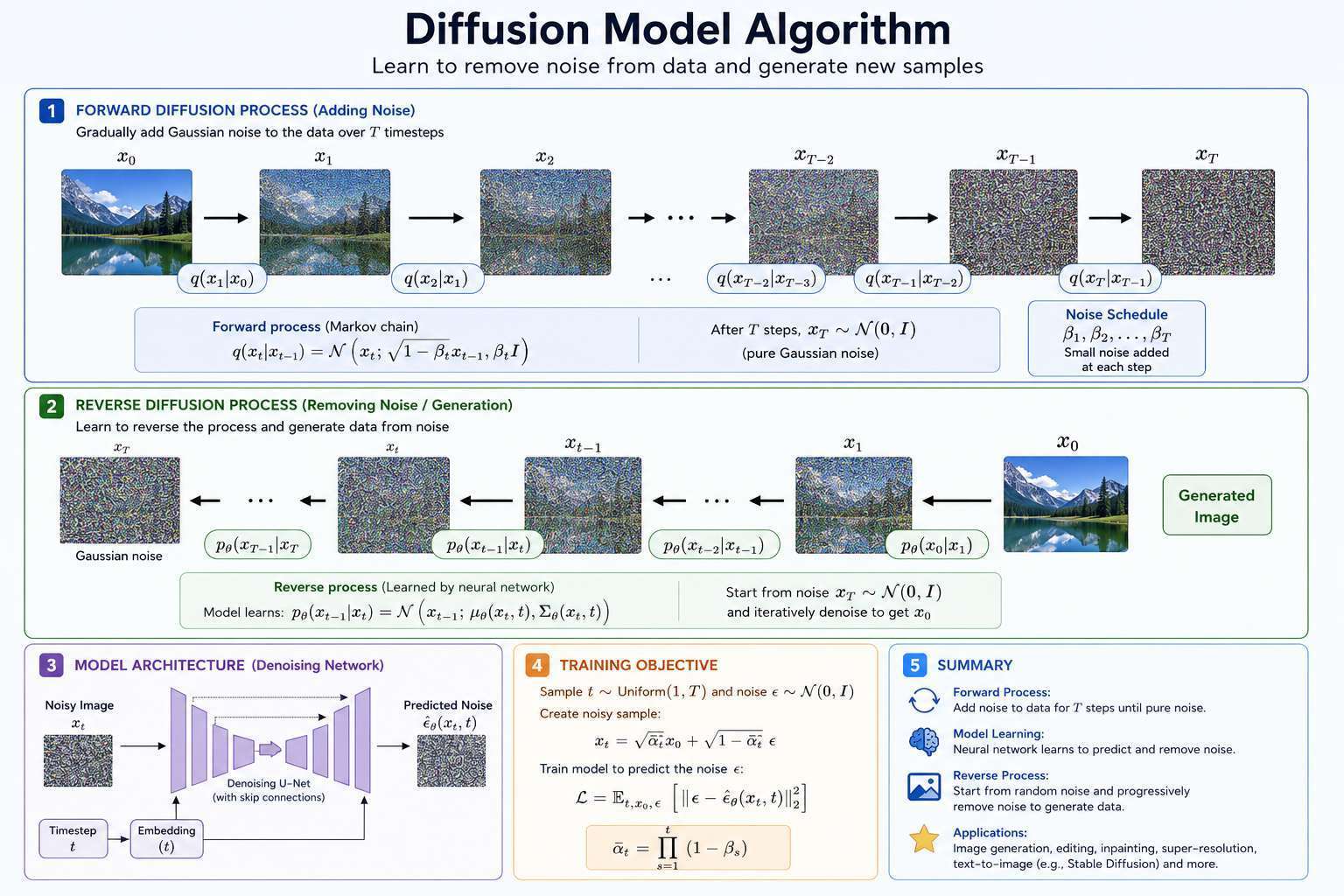
What Are Diffusion Models?

A diffusion model learns to generate images by reversing a process that gradually corrupts images with noise.

The idea is surprisingly simple:

graph LR

    Image[Image Data]
    Image --> AddNoise
    AddNoise --> PureNoise

Then train a neural network to reverse the process:

graph LR

    PureNoise
    PureNoise --> RemoveNoise
    RemoveNoise --> LessNoise
    LessNoise --> Image

The model learns how to transform random noise into realistic images.

Training follows these steps:

graph TD

    CleanImage

    --> AddNoise

    --> NoisyImage

    --> UNet

    --> PredictNoise

    --> Loss

For every training image:

• Sample a timestep
• Add noise
• Predict noise
• Compute loss
• Update weights

The model gradually learns how noise behaves.

---

Inspiration from Physics

The term "diffusion" comes from physical diffusion processes.

Imagine dropping ink into water.

Initially:

Ink Drop

Over time:

Ink + Water

Eventually:

Uniform Mixture

Information becomes increasingly dispersed.

Diffusion models apply a similar concept to images.

---

The Forward Diffusion Process

The forward process gradually adds noise to an image.

graph TD

    Image[Original Image]
    SlightNoise[Slight Noise]
    MoreNoise[More Noise]
    HeavyNoise[Heavy Noise]
    RandomNoise[Random Noise]

    Image --> SlightNoise --> MoreNoise--> HeavyNoise --> RandomNoise


    A[Original Image]

    A--> B[10% Noise]
    B --> C[30% Noise]
    C --> D[60% Noise]
    D --> E[100% Noise]

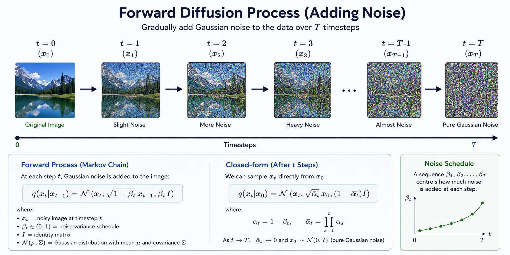
At each step:

$$x_t = \sqrt{1-\beta_t} x_{t-1}+ \sqrt{\beta_t} \epsilon$$

Where:

• $x_t$ = image at timestep $t$
• $\beta_t$ = noise schedule
• $\epsilon$ = Gaussian noise

After enough steps:

$$x_T \approx \mathcal{N}(0, I)$$

The image becomes pure noise.

---

The Reverse Diffusion Process

The real magic happens during reverse diffusion.

Starting with random noise:

graph TD

    Noise[Random Noise]
    LessNoise[Less Noise]
    Shape[Emerging Shape]
    Structure[More Structure]
    FinalImage[Final Image]

    Noise --> LessNoise--> Shape--> Structure--> FinalImage

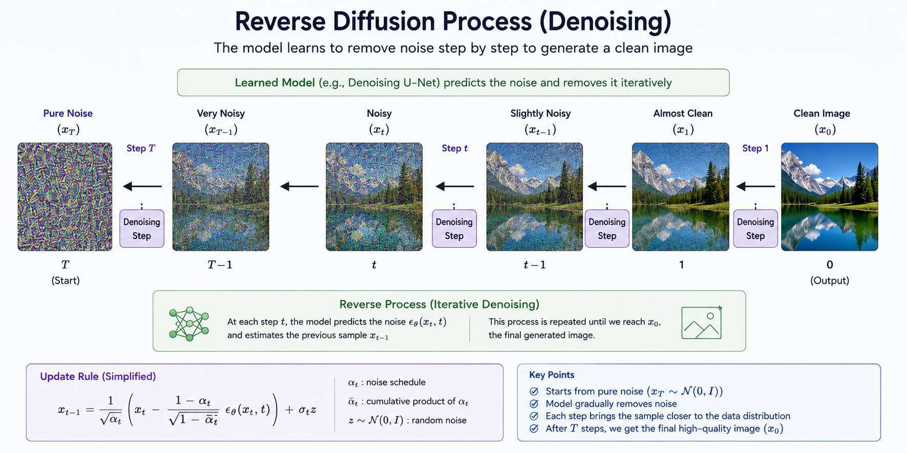
The model predicts what noise should be removed at each step.

Learning to Predict Noise

Instead of directly generating images, diffusion models learn to predict noise.

Input:

$x_t$ : the noisy image at timestep $t$

Output:

$\hat{\epsilon}$ : the predicted noise

Architecture:

graph LR

    NoisyImage[Noisy Image]
    UNet[U-Net Algorithm]
    PredictedNoise[Predicted Noise]

    NoisyImage --> UNet --> PredictedNoise

The network learns:

What part is noise?
What part is signal?

Why Predict Noise?

Predicting noise is easier than predicting the entire image.

The training objective becomes:

$$Loss = ||\epsilon - \hat{\epsilon}||^2$$

Where:

• $\epsilon$ = actual noise
• $\hat{\epsilon}$ = predicted noise

This Mean Squared Error (MSE) objective is stable and effective.

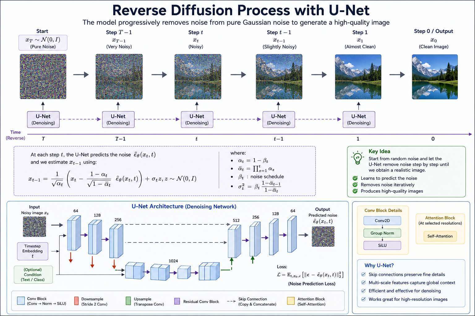
Generating Images With UNet

Once trained:

1. Start with random noise
2. Run reverse diffusion
3. Remove noise step by step
4. Obtain an image

graph TD

    Noise --> Step_1--> Step_2--> Step_n--> Image

This process can involve hundreds of denoising steps.

The Role of U-Net

Most diffusion models use a U-Net architecture.

graph TD

    Input[Noisy Image]

    Input--> Encoder --> Bottleneck --> Decoder--> Output[Predicted Noise]

    Encoder -. Skip Connections .-> Decoder

Why U-Net?

• Captures global context
• Preserves fine image details
• Works at multiple scales
• Excellent for denoising tasks

Mathematical Objective

The model approximates:

$$p(x_{t-1}|x_t)$$

which represents:

How likely is the previous image
given the current noisy image?

By repeatedly applying this estimate, the model reconstructs images.

---

Conditional Diffusion Models

Modern systems generate images from prompts.

Example:

A futuristic city at sunset

Architecture:

graph TD

    Prompt --> TextEncoder--> Embedding--> DiffusionModel--> Image

The text embedding guides the denoising process.

CLIP and Diffusion

Many systems use CLIP-based text encoders.

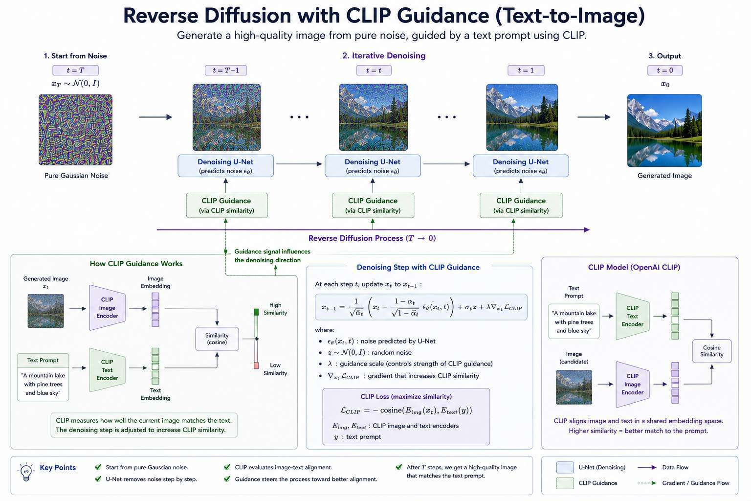
Workflow:

graph TD

    TextPrompt[Text Prompt]
    CLIP[CLIP Text Encoder]
    TextEmbedding[Text Embedding]
    UNet[U-Net Denoiser]
    GeneratedImage[Generated Image]
   

    TextPrompt --> CLIP --> TextEmbedding --> UNet --> GeneratedImage
    

The text embedding tells the model:

What should be generated?

The U-Net determines:

How should it look?

---

Latent Diffusion Models

Running diffusion directly on high-resolution images is expensive.

Instead of operating on images directly, the model operates on latent representations.

Stable Diffusion introduced:

$$Latent\ Diffusion$$

Latent Space

Latent space (also called embedding space) is a compressed, abstract representation of data used by AI and machine learning models

graph TD

    Image--> Encoder --> LatentSpace

So Architecture Becoemes:

graph TD

    Image --> Encoder--> LatentSpace --> DiffusionModel --> Decoder--> GeneratedImage

Benefits:

• Faster training
• Lower memory requirements
• Higher resolutions

---

Why Diffusion Models Replaced GANs

GANs consist of:

Generator
vs
Discriminator

Training can be unstable.

Problems include:

• Mode collapse
• Training instability
• Difficult optimization

Diffusion models offer:

• Stable training
• Better diversity
• Higher image quality
• Strong prompt alignment

GANs vs Diffusion Models

Feature	GANs	Diffusion Models
Training Stability	Medium	High
Image Quality	High	Very High
Diversity	Medium	High
Prompt Control	Limited	Excellent
Training Complexity	High	Medium
Generation Speed	Fast	Slower

---

Applications of Diffusion Models

Text-to-Image Generation

Examples:

• Stable Diffusion
• Midjourney
• DALL·E

Image Editing

Tasks:

• Inpainting
• Outpainting
• Style transfer

Video Generation

Generate videos from:

• Text prompts
• Images
• Existing videos

Medical Imaging

Applications:

• MRI reconstruction
• Image enhancement
• Synthetic data generation

Scientific Research

Generate:

• Molecular structures
• Protein conformations
• Material simulations

---

Challenges

Despite their success, diffusion models have limitations.

1. Slow Inference

Generating an image may require:

20–100 denoising steps

or more.

2. High Compute Requirements

Training large diffusion models often requires:

• Multiple GPUs
• Large datasets
• Significant storage

3. Prompt Sensitivity

Small prompt changes can produce dramatically different outputs.

Future of Diffusion Models

Research is focused on:

• Faster sampling
• Video diffusion
• 3D diffusion
• Audio diffusion
• Real-time generation

Emerging architectures are reducing generation times from minutes to seconds.

---

Final Thoughts

Diffusion models have fundamentally changed Generative AI.

Their core idea is elegant:

$$Image \rightarrow Noise \rightarrow Image$$

Training teaches the model how noise is added.

Generation teaches the model how noise is removed.

The workflow can be summarized as:

$$Forward\ Diffusion + Reverse\ Diffusion = Image\ Generation$$

Combined with U-Net architectures and powerful text encoders, diffusion models have become the foundation of modern image generation systems.

From creating art and videos to scientific discovery and medical imaging, diffusion models represent one of the most important breakthroughs in contemporary AI.