Normal Equation in Linear Regression: Formula, Intuition, and Comparison with Gradient Descent

Normal Equation (Closed-Form Solution)

Instead of solving multiple iteration of gradient descent, Normal equation can get theta in one step

• Θ can be directly calculated where cost function is minimal using calculus in one step instead of iterating iterative optimization:

$$\theta = (X^T X)^{-1} X^T y$$

Advantages

• No learning rate required
• Direct computation

Limitations

• Computationally expensive for very large datasets
• Matrix inversion can be costly

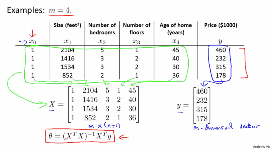
Steps:

• Construct design matrix X using feature columns and add 1 in first column
• Construct y vector using result values Y
• calculate:

Θ = (XTX)-1 XTy

Feature scaling is not required for Normal Equation method

Normal Equation vs Gradient Descent:

Feature	Gradient Descent	Normal Equation
Complexity	Complex need to debug alpha	Convenient & Simple to implement
Choose Learning Rate(α)	Required	No need
Feature Scaling	Required	No need
Iteration	Many Iteration Required	Not required
Feature Set>=million	Efficient if n is huge O(kn2)	Slow if n is huge, cost of inverse matrix is O(n3)
Complex Learning Algo	Can used for Complex learning algo	Not supported

---

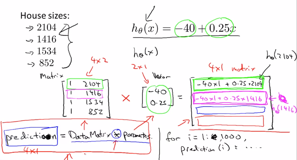
Faster single Hypothesis Prediction calculation given data set and Thetas **Much faster than nested for loops

Data Matrix * Parameter Vector = Prediction Vector

h(x) = Theta0 + Theta1x
[1 , x]*[Theta Vector] = [h(x)]

Usage:

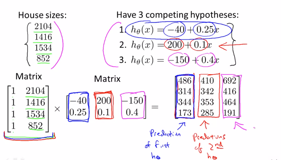
• Faster multiple Hypothesis Prediction calculation given data set and Thetas
• Much-much faster than nested for loops

Data Matrix * Parameter Matrix = Prediction Matrix

  given h(x) = Theta0 + Theta1x

  [1 , x]*[Theta Matrix] = [h(x)]

---

Normal Equation with Regularization

Instead of iterative gradient descent, we can use the normal equation.

Without Regularization:

$$\theta = (X^T X)^{-1} X^T y$$

With Regularization (Ridge Regression):

$$\theta = (X^T X + \lambda L)^{-1} X^T y$$

This discourages large parameter values and reduces overfitting.

Where Matrix $L$

$$L = \begin{bmatrix} 0 & 0 & 0 & \cdots & 0 \\ 0 & 1 & 0 & \cdots & 0 \\ 0 & 0 & 1 & \cdots & 0 \\ \vdots & \vdots & \vdots & \ddots & \vdots \\ 0 & 0 & 0 & \cdots & 1 \end{bmatrix}$$

Properties:

• It is almost the identity matrix except the top-left element is 0.
• Dimension: $(n+1) \times (n+1)$

First diagonal entry is 0 because no regularization for $\theta_0$

Remaining diagonal entries are 1 because we regularize $\theta_1$ to $\theta_n$.

$$L = \text{diag}(0,1,1,\dots,1)$$

This ensures:

• $\theta_0$(bias term) is not regularized
• All other parameters are regularized

---

Why Regularization Helps

If $m < n$, then $X^T X$ is non-invertible.
If $m = n$, it may or may not be invertible.

where

• $m$ = number of training examples
• $n$ = number of features

In other terms if $m < n$, then:

$$X^T X$$

is non-invertible.

However, with regularization we add $\lambda L$ to $X^T X$:

$$X^T X + \lambda L$$

That makes whole term invertible (for $\lambda > 0$).

This improves numerical stability.

---