Cost Function Regularization: Balancing Bias and Variance in Machine Learning Models

Regularization 🛑

If a model is overfitting, we can reduce the influence of certain terms by increasing their cost. This discourages large weights.

Regularization balances:

• Bias
• Variance

Regularization techniques

Used to make reduce variance and solve problem of Overfitting

• Instead of removing features, keep them all but reduce parameter sizes.

• Regularization adds a penalty term to the cost function to discourage complexity.

• Regularization helps prevent overfitting by keeping the model simpler.

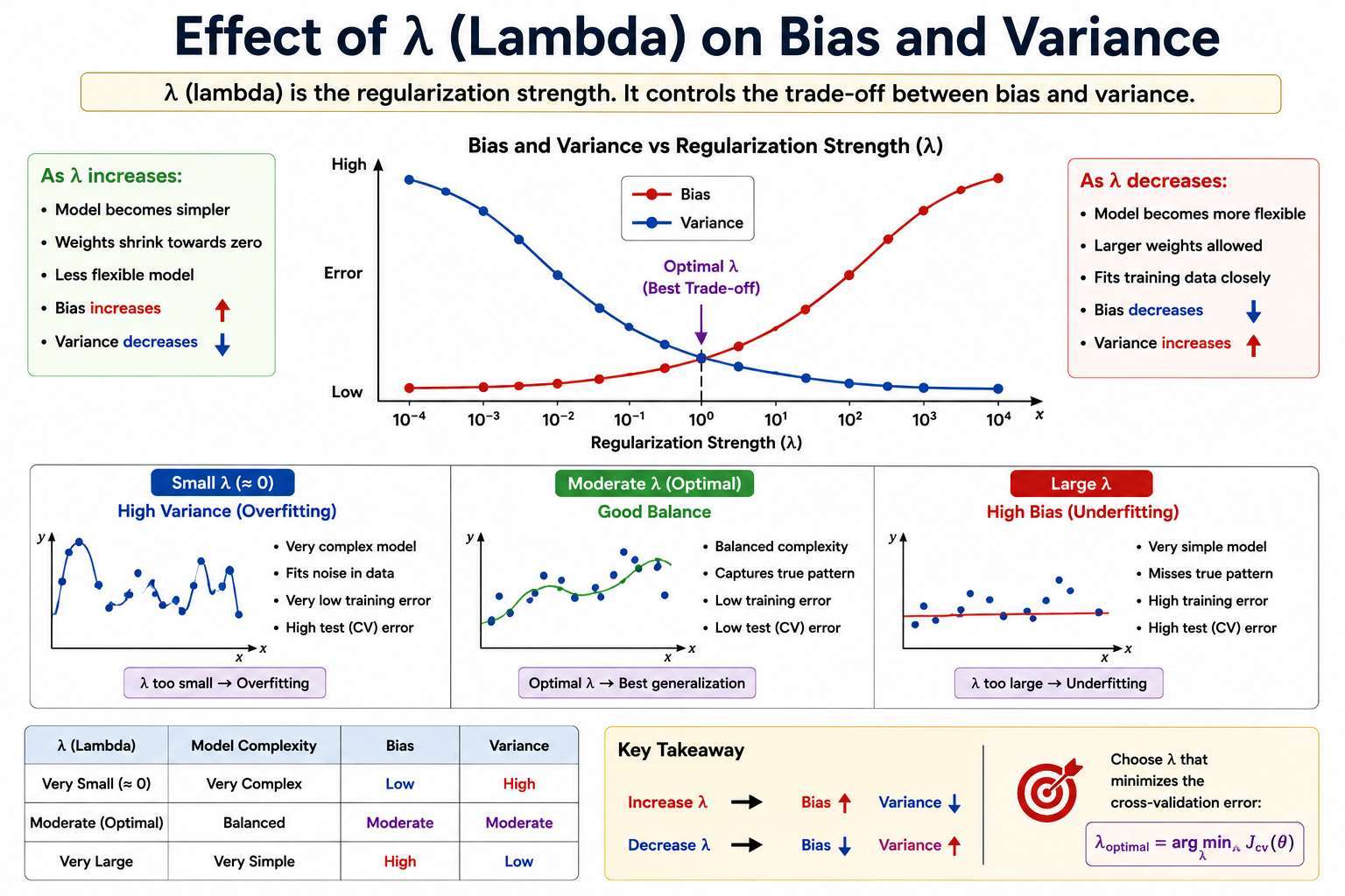
• The regularization parameter λ controls the strength of the penalty. A larger λ means more regularization.

Instead of removing features, keep them all but reduce parameter sizes.

The idea:

• Large weights → complex model
• Small weights → smoother model

---

General Regularized Cost Function

In standard linear regression, the cost function is:

Mean Squared Error

Measures how well the model fits the training data.

$$J(\theta) = \frac{1}{2m} \sum_{i=1}^{m} (h_\theta(x^{(i)}) - y^{(i)})^2$$

We Add Regularization Term to it

Regularization term

Penalizes large parameter values to prevent overfitting.

The Regularization term is:

$$\lambda \sum_{j=1}^{n} \theta_j^2$$

• $\lambda$ is the regularization parameter that controls the strength of regularization.
• This term penalizes large values of $\theta_j$, encouraging smaller weights and thus simpler models.

The parameter vector contains:

$$\theta_1, \dots, \theta_n$$

Explicitly excludes the bias term $\theta_0$.

• Regularization runs from $j = 1$ to $n$
• So $\theta_0$ is not penalized

Why Exclude $\theta_0$?

The bias term controls the decision boundary shift.

We do not want to shrink it toward zero.

Only the other parameters are regularized.

So effective cost become

$$J(\theta) = \min_\theta \; \frac{1}{2m} \sum_{i=1}^{m} \left( h_\theta(x^{(i)}) - y^{(i)} \right)^2+ \lambda \sum_{j=1}^{n} \theta_j^2$$

We can regularize all parameters using a single summation over $j=1$ to $n$

We dont regularized Bias parameter $\theta_0$

Regularization Algos

Lasso vs Ridge

Feature	Lasso (L1) 🔹	Ridge (L2)
Penalty	Sum of absolute values $\sum \| \theta_j\|$	Sum of squares $\sum \theta_j^2$
Effect	Can shrink some coefficients exactly to 0 → feature selection	Shrinks coefficients but rarely to 0
Use Case	Many irrelevant features	Prevent overfitting, keep all features

1. Lasso Regression (L1 Regularization) 🔹

Lasso: Cost = MSE + λ * sum(|θ|)

• Lasso (L1) can shrink some coefficients to zero, effectively performing feature selection.

Lasso adds a penalty proportional to the sum of absolute values of the coefficients:

$$J(\theta) = \frac{1}{2m} \sum_{i=1}^{m} (h_\theta(x^{(i)}) - y^{(i)})^2 + \lambda \sum_{j=1}^{n} |\theta_j|$$

Where:

• $\lambda$ = regularization strength
• $|\theta_j|$ = absolute value of parameter $\theta_j$
• $\theta_0$ (bias) is usually not penalized

2. Ridge Regression (L2 Regularization) 🏔️

Ridge: Cost = MSE + λ * sum(θ^2)

• Ridge (L2) shrinks coefficients but does not set them to zero.

Ridge adds a penalty proportional to the sum of squared coefficients:

$$J(\theta) = \frac{1}{2m} \sum_{i=1}^{m} (h_\theta(x^{(i)}) - y^{(i)})^2 + \lambda \sum_{j=1}^{n} \theta_j^2$$

Where:

• $\lambda$ = regularization strength
• $\theta_j$ = model parameters
• $\theta_0$ (bias) is usually not penalized

---

Regularization Parameter $\lambda$

Regularization shrinks parameters. The more shrinkage you see, the larger the $\lambda$

Choosing $\lambda$ correctly is essential for good generalization.

The regularization parameter λ (lambda) controls the tradeoff between bias and variance.

Lambda (λ)	Model Complexity	Bias	Variance
Very Small (0)	Very Complex	Low	High
Moderate	Balanced	Moderate	Moderate
Very Large	Very Simple	High	Low

Larger $\lambda$ → stronger regularization

$\lambda \to \infty$ → all parameters shrink to zero → model becomes too simple → underfitting

• Parameter Weights $\theta_j$ shrink toward zero
• Reduces model complexity and make it rigid/linear
• Underfitting may occur
  • Bias increases
  • Variance decreases

Example:

$\lambda = 1 => \theta =[ 13.01, 0.91]$

Smaller $\lambda$ (as $λ → 0$)

$\lambda \to 0$ → no regularization → model may overfit

weaker regularization --> Less Penalty --> Large weights $\theta_j$

• Parameter weights grow larger
• More complex models & becomes more flexible/curvy
• Risk of overfitting
  • Variance increases
  • Bias decreases

Small λ → Low bias, high variance (overfitting)

Example:

$\lambda = 0.01 => \theta =[ 81.01, 12.00]$

What Happens If $\lambda = 0$?

• No regularization is applied
• The model may overfit
• We revert to standard least squares / logistic regression

---

How to Choose the Best λ

To select the optimal regularization parameter:

1. Choose candidate λ values
2. Train models for each λ
3. Compute cross-validation error (without regularization)
4. Select best λ + model
5. Evaluate once on test set

1. Create Candidate Values

Example:

$$\lambda \in \{0, 0.01, 0.02, 0.04, 0.08, 0.16, 0.32, 0.64, 1.28, 2.56, 5.12, 10.24\}$$

2. Train Models

For each value of λ:

• Train model parameters Θ
• Possibly try different model complexities (degrees, architectures, etc.)

3. Compute Cross-Validation Error

Evaluate using:

$$J_{CV}(\Theta)$$

Important:

• Compute cross-validation error without regularization
• That means use λ = 0 when evaluating

This ensures fair comparison between models.

4. Select Best Combination

Choose the model and λ that produce the lowest cross-validation error.

5. Final Evaluation

Using the best:

• Θ
• λ

Evaluate on the test set:

$$J_{test}(\Theta)$$

This measures generalization performance.

---

Example: Polynomial Hypothesis

Consider the function:

$$\theta_0 + \theta_1 x + \theta_2 x^2 + \theta_3 x^3+ \theta_4 x^4$$

If we want the model to behave more like a quadratic function, we can reduce the influence of:

$$\theta_3 x^3 \quad \text{and} \quad \theta_4 x^4$$

Instead of removing these features, we modify the cost function.

Regularized Cost Function

We minimize:

$$\min_\theta \; \frac{1}{2m} \sum_{i=1}^{m} \left( h_\theta(x^{(i)}) - y^{(i)} \right)^2 + 1000 \theta_3^2 + 1000 \theta_4^2$$

Effect of Large Penalty

Adding large penalty terms forces:

$$\theta_3 \approx 0 \quad \text{and} \quad \theta_4 \approx 0$$

This reduces the contribution of:

$$\theta_3 x^3 \quad \text{and} \quad \theta_4 x^4$$

As a result:

• The hypothesis becomes smoother
• Overfitting decreases
• The curve behaves more like a quadratic function

---

---

Related Posts

• Cost Function for Neural Networks — the neural network cost function contains the same L2 regularization term (summed over all layers); the math is identical, just applied at scale
• Bias-Variance Dilemma — regularization is the main lever for moving from high variance (overfitting) toward the bias-variance sweet spot
• Polynomial Regression — where high-variance overfitting — and the need for regularization — shows up most visibly